Lab 14: ANCOVA

About

Here we go for our final linear-model example. It is unique in that it combines a categorical explanatory variable with a continuous explanatory variable. What are we up to? We are combining regression and one-way ANOVA! Yes we are.

ANCOVA

This week, we will be using the lm() function to fit a linear regression to data which has a continuous AND a categorical variable. Essentially, we will be fitting two linear regression models (one for each level of the categorical variable), and testing whether these lines are different from each other or not.

Preliminaries

Packages

For this lab, we will be using the dplyr, ggplot2, and Sleuth3 packages. Make sure all packages are installed on your computer (you may need to install Sleuth3), and then run the following code:

library(tidyverse)
library(Sleuth3)

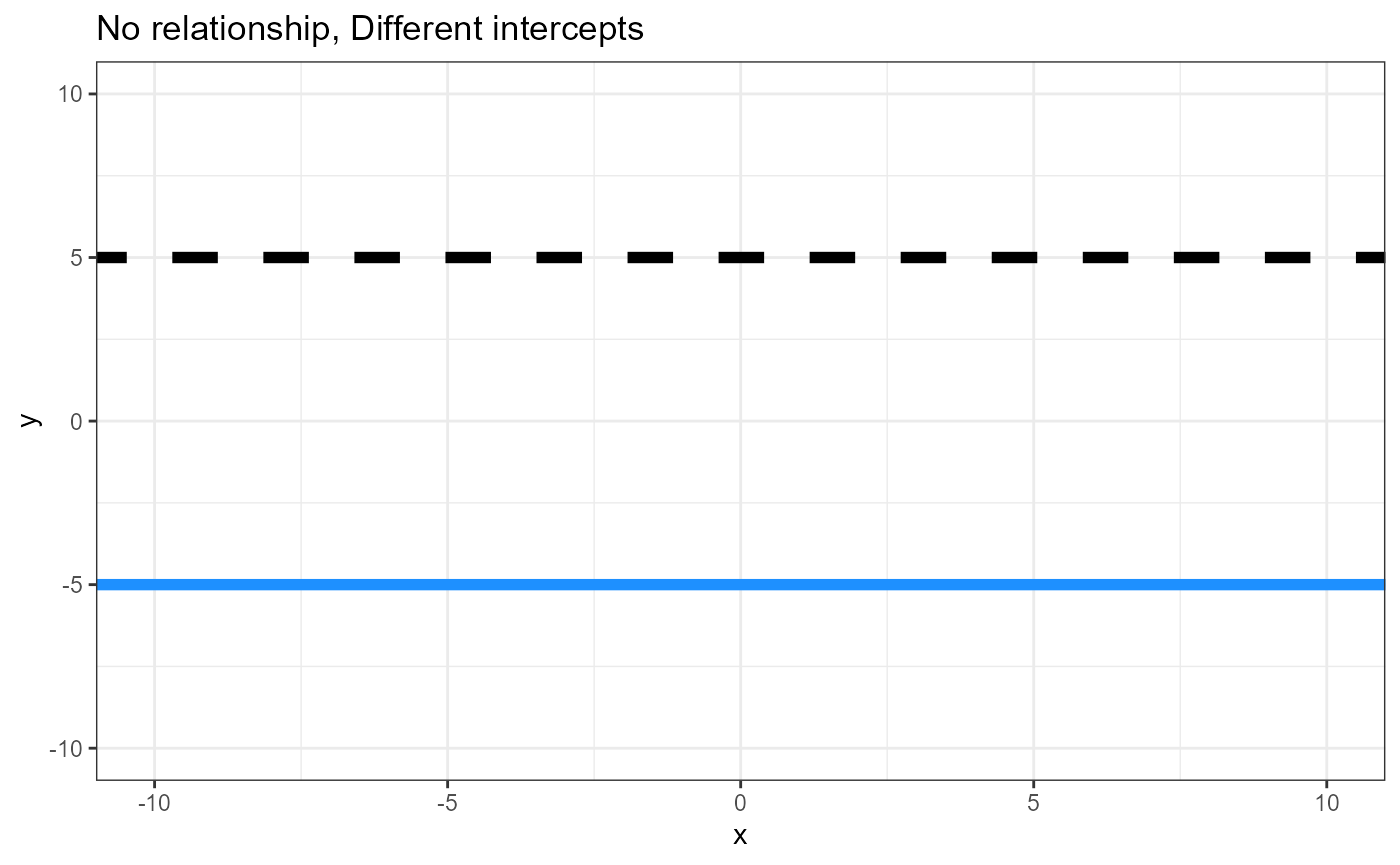
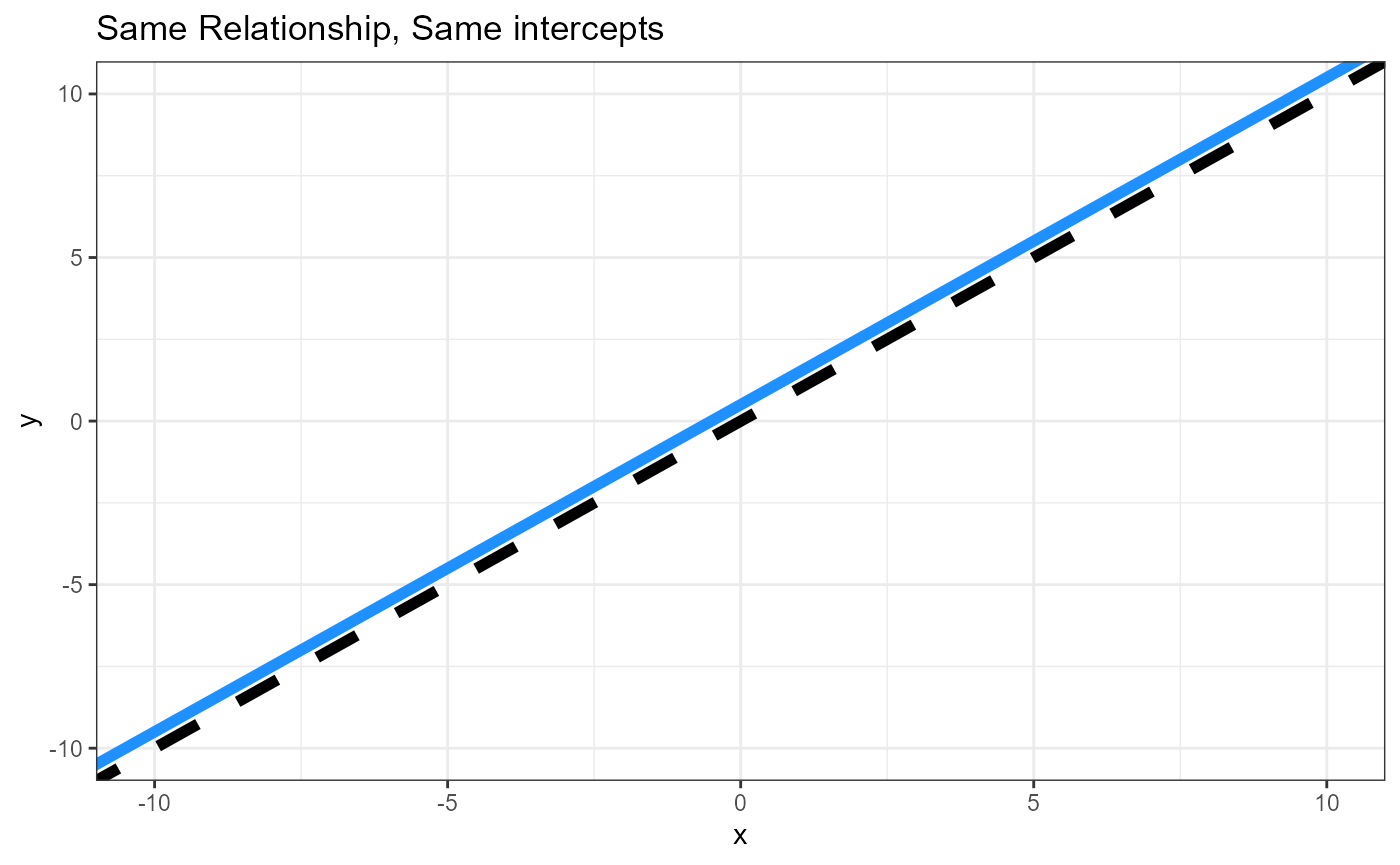
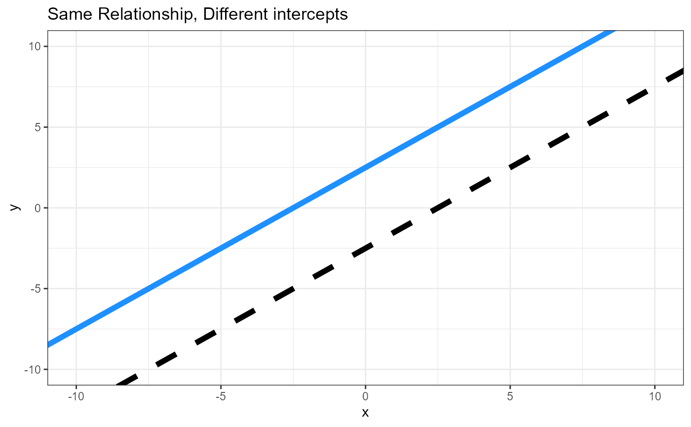
Hypotheses, plain words

Is the intercept for the reference level = 0?
Is there a difference in intercepts between the groups (Think ANOVA)
Is there a relationship between the response and continuous predictor variable regardless of groups? (Think a “global” linear regression, ignoring/averaging across groups)
Does the relationship between the response and continous predictor differ between groups? i.e., are the slopes different?

Hypotheses, graphs

## Warning: Using `size` aesthetic for lines was deprecated in ggplot2 3.4.0.
## ℹ Please use `linewidth` instead.
## This warning is displayed once every 8 hours.
## Call `lifecycle::last_lifecycle_warnings()` to see where this warning was
## generated.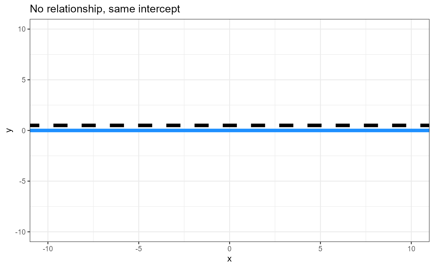

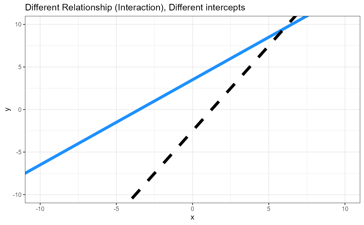
Parameters, two linear equations

Equation for the line of the reference (REF) level

\[\hat{y}_{REF} = \beta_0 + \beta_1*x_1\]

Equation for the line of the alternative (ALT) level

\[\hat{y}_{ALT} = (\beta_0 +\beta_{0\Delta}) + (\beta_1 +\beta_{1\Delta})*x_1\]

\(\Delta\) is the Greek letter Delta, and is commonly used to represent differences
\(\beta_0\) = intercept for reference level
\((\beta_{0\Delta})\) = Difference between intercepts
\(\beta_1\) = Slope for reference level
\((\beta_{1\Delta})\) = Difference between slopes (Interactive effect)

NOTE We are keeping things simple with just two levels of the categorical variable. For each additional level, \(i\), there will be two more parameters estimated in the linear model, one each for the difference in intercepts between the reference level and level \(i\) (\(\beta_{0\Delta_i}\), and one for the difference in slopes between the reference level and level \(i\) (\(\beta_{1\Delta_i}\).

Data

We will be using a data set from the Sleuth3 package called case1402 . This is data from an experiment examining the yield of different soybean varieties under different conditions of Ozone, SO2 and drought. See ?case1402 for more information.

Load data and rename object

df <- case1402

head(df)

##         Stress  SO2   O3 Forrest William
## 1 Well-watered 0.00 0.02    4376    5561
## 2 Well-watered 0.00 0.05    4544    5947
## 3 Well-watered 0.00 0.07    2806    4273
## 4 Well-watered 0.00 0.08    3339    3470
## 5 Well-watered 0.00 0.10    3320    3080
## 6 Well-watered 0.02 0.02    3747    5092

William: Response variable, continuous, needs to be log() transformed
O3: Predictor variable, continuous
Stress: Predictor variable, categorical/factor
- Levels: Stressed, Well-watered

Transform `William` variable

df <- df %>%
  mutate(log_william = log(William))

Plot data

Scatterplot with continuous x- and y-variables.

ggplot(df,
       aes(x = O3, 
           y = log_william)) +
  geom_point() +
  theme_bw()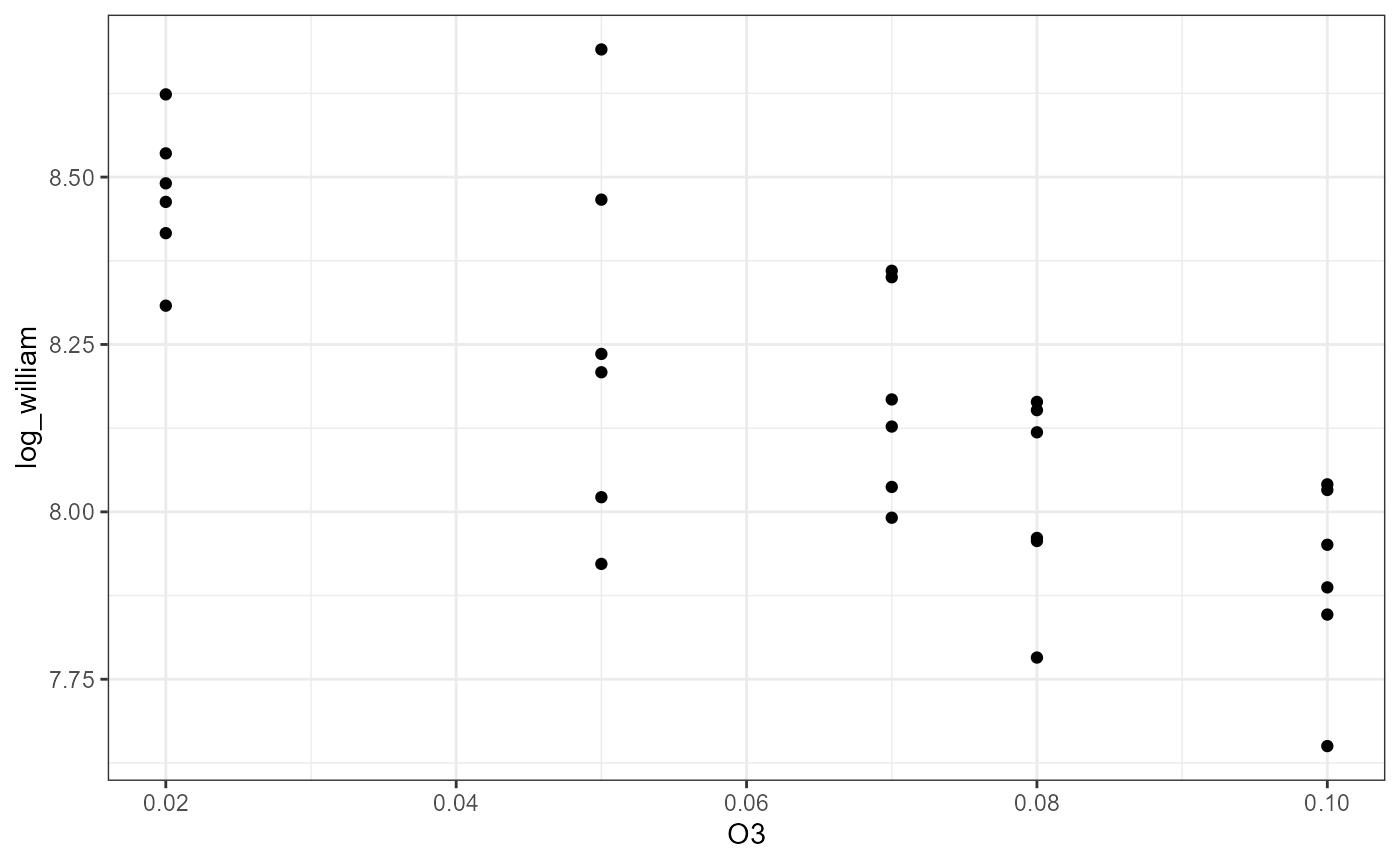

ggplot(df,
       aes(x = O3, 
           y = log_william)) +
  geom_point() +
  theme_bw() +
  geom_smooth(method = "lm")

## `geom_smooth()` using formula = 'y ~ x'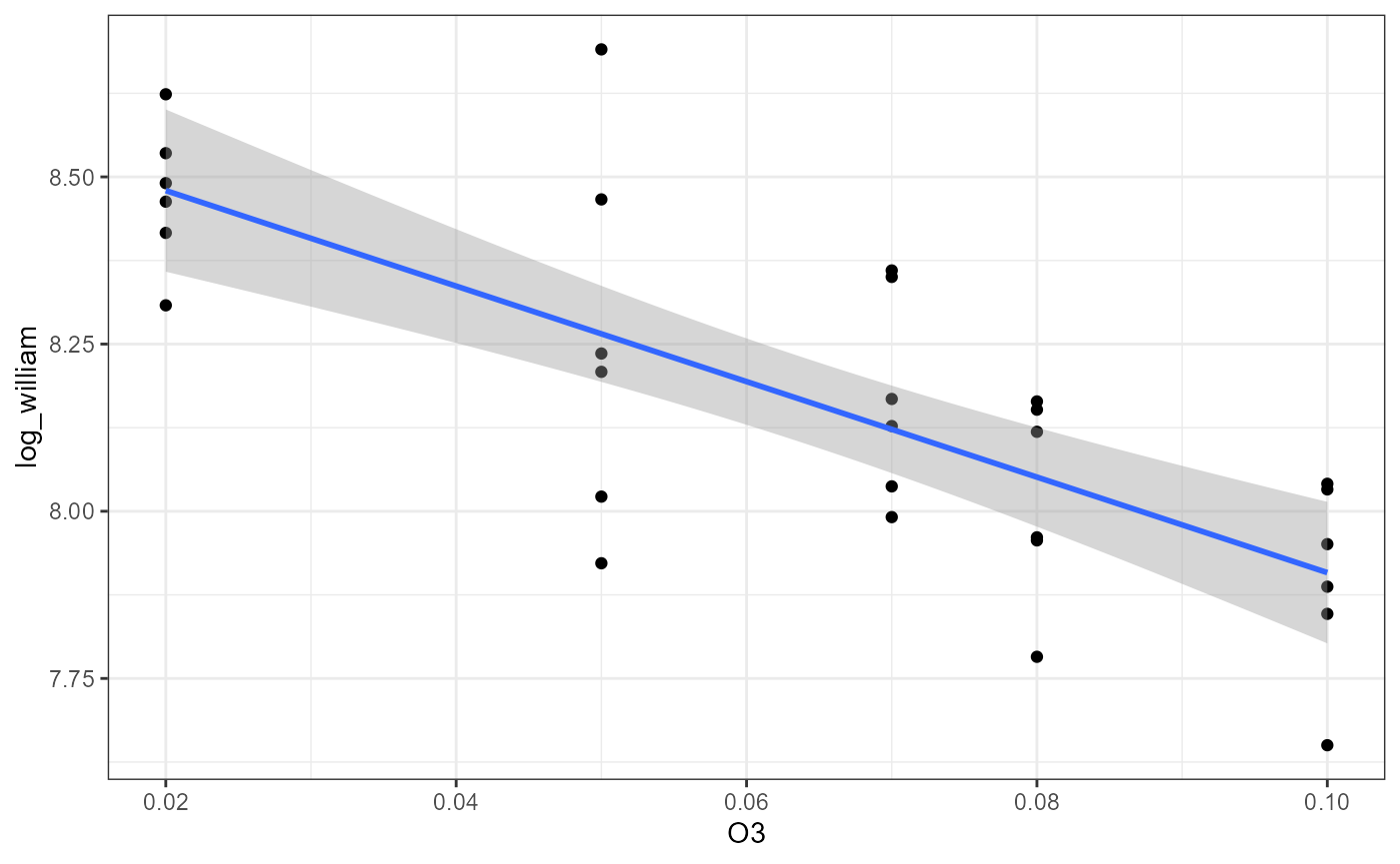

### Factor

ggplot(df, 
       aes(y = log_william, 
           x = Stress,
           color = Stress)) +
  geom_boxplot() +
  geom_point(position = position_jitter(width = 0.1, height = NULL)) +
  theme_bw()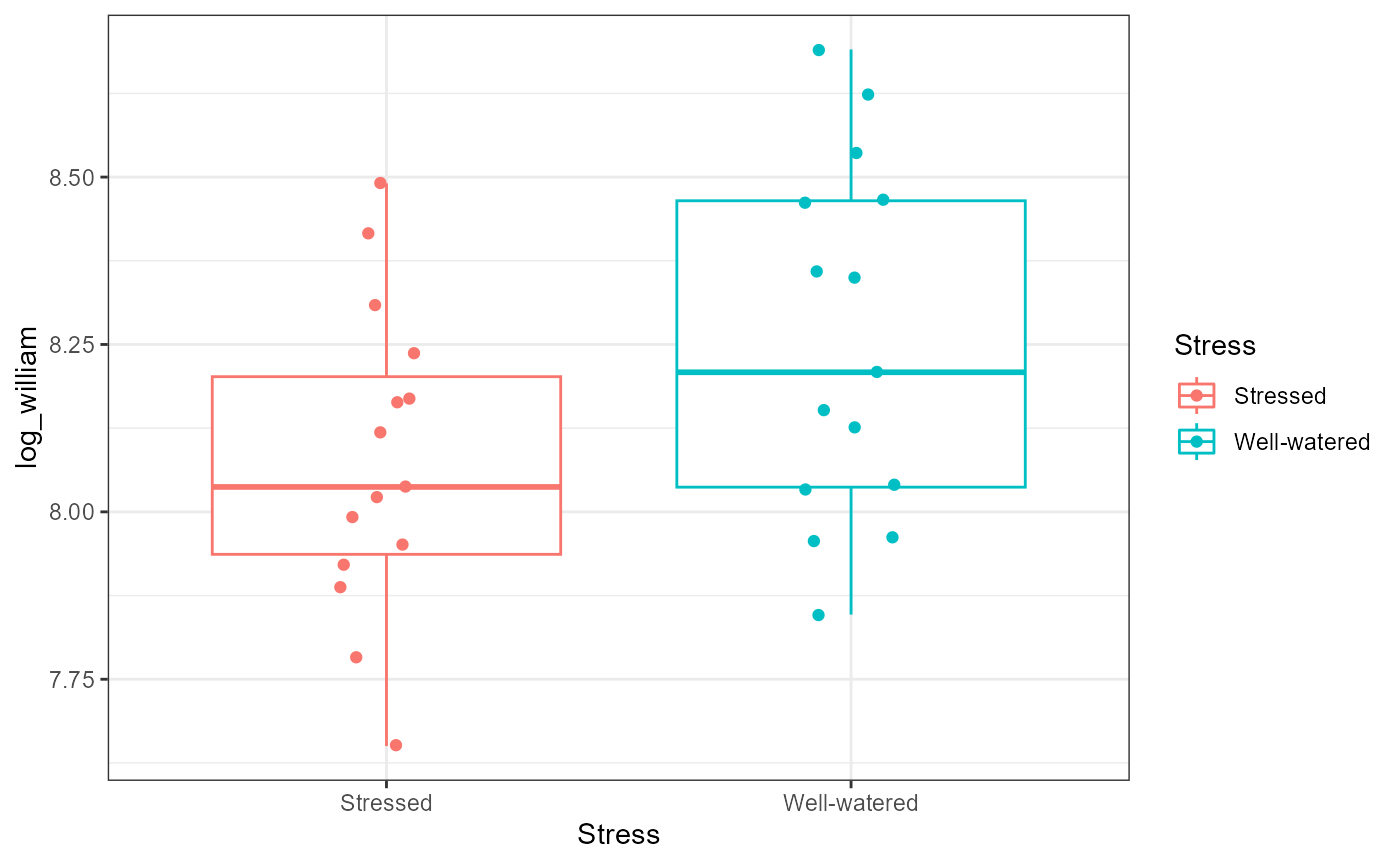

Plot both predictor variables

ggplot(df,
       aes(x = O3, 
           y = log_william,
           color = Stress)) +
  geom_point() +
  theme_bw()

#### With geom_smooth()

ggplot(df,
       aes(x = O3, 
           y = log_william,
           color = Stress,
           fill = Stress)) +
  geom_point() +
  theme_bw() +
  geom_smooth(method = "lm")

## `geom_smooth()` using formula = 'y ~ x'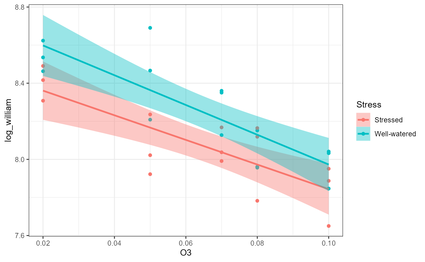

Fit ANCOVA model

df_lm <- lm(log_william ~ O3 * Stress, data = df)

Assumptions

ggplot(df, 
       aes(sample = log_william)) +
  stat_qq() +
  stat_qq_line()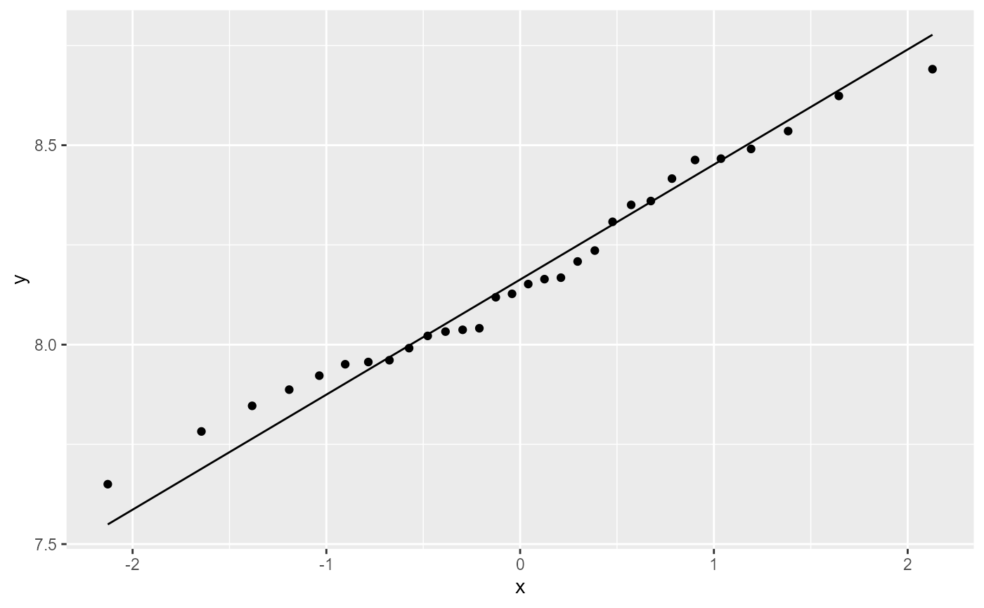

ggplot(df_lm, 
       aes( x = .fitted, 
            y = .resid)) +
  geom_point()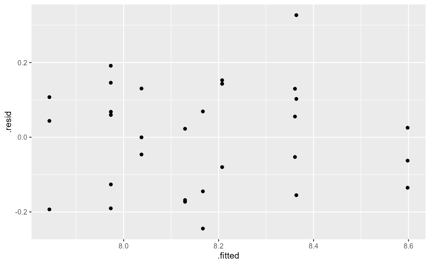

ANOVA table

anova(df_lm)

## Analysis of Variance Table
## 
## Response: log_william
##           Df  Sum Sq Mean Sq F value    Pr(>F)    
## O3         1 1.13812 1.13812 51.9277 1.185e-07 ***
## Stress     1 0.23764 0.23764 10.8426  0.002859 ** 
## O3:Stress  1 0.01013 0.01013  0.4621  0.502639    
## Residuals 26 0.56985 0.02192                      
## ---
## Signif. codes:  0 '***' 0.001 '**' 0.01 '*' 0.05 '.' 0.1 ' ' 1

Interpretation: There is a significant main effect of O3 (\(F_{1, 26} = 51.92\), \(p < 0.001\)) and a significant main effect of Stress (\(F_{1, 26} = 10.84\), \(p = 0.002\)). There was no significant interactive effect (\(F_{1, 26} = 0.46\), \(p = 0.5\)).

Plain words: There was a relationship between yield ( log_william ) and O3 (continuous predictor variable). Likewise, there was a difference in average yield based on the Stress factor (categorical predictor variable, different intercepts for each group). The relationship between yield and ozone was not dependent on the stress factor, and vice versa (both groups had the same slope).

Linear model summary

summary(df_lm)

## 
## Call:
## lm(formula = log_william ~ O3 * Stress, data = df)
## 
## Residuals:
##      Min       1Q   Median       3Q      Max 
## -0.24461 -0.13302  0.02398  0.10615  0.32690 
## 
## Coefficients:
##                       Estimate Std. Error t value Pr(>|t|)    
## (Intercept)             8.4902     0.0975  87.083  < 2e-16 ***
## O3                     -6.4672     1.4014  -4.615 9.29e-05 ***
## StressWell-watered      0.2642     0.1379   1.916   0.0664 .  
## O3:StressWell-watered  -1.3473     1.9819  -0.680   0.5026    
## ---
## Signif. codes:  0 '***' 0.001 '**' 0.01 '*' 0.05 '.' 0.1 ' ' 1
## 
## Residual standard error: 0.148 on 26 degrees of freedom
## Multiple R-squared:  0.7086, Adjusted R-squared:  0.675 
## F-statistic: 21.08 on 3 and 26 DF,  p-value: 3.899e-07

Equation for line 1: `Stressed`

\[Yield_{Stressed} = \beta_0 + \beta_1 * \text{Ozone} \]

(Intercept) \(\beta_0\): Estimate = 8.49; This is the average yield for the Stressed treatment when Ozone = 0.
O3 \(\beta_1\): Estimate = -6.47; For every 1-unit increase in Ozone, the average yield changes by -6.47.
#### Full equation

\[ \text{Yield}_{Stressed} = 8.49 - 6.47 * \text{Ozone}\]

Equation for line 2: `Well-watered`

\[Yield_{well-watered} = (\beta_0+\beta_{0 \Delta}) + (\beta_1 +\beta_{1 \Delta}) * \text{Ozone} \]

StressWell-watered: This is the estimated difference (\(\beta_0+\beta_{0 \Delta}\)) in intercepts for the two treatment groups. Estimate = \(\beta_0 + \beta_{well-watered} = 8.49 + 0.2642 = 8.75\); This is the average yield for the Well-watered treatment when Ozone = 0.
O3:Stresswell-watered: This is the estimated difference (\(\beta_1 +\beta_{1 \Delta}\)) in slopes for the two treatment groups (but note that the p-value > 0.05, so we fail to reject the NULL that this coefficient is 0). Estimate = \(-6.47 - 1.35 = -7.82\).

\[ \text{Yield}_{well-watered} = (8.49 + 0.2642) - (6.47 - 1.35) * \text{Ozone} = 8.75 - 7.82 * \text{Ozone}\]

Note that these equations will be slightly different from what geom_smooth(method = "lm") will estimate. To see how to plot the estimated model fits in ggplot, see the appendix of this lab.

Coda

This concludes lab 08

Appendix: Plotting model estimates

Make a new data frame with values of predictor variables

new_x <- expand.grid(
  O3 = seq(from = min(df$O3),
           to = max(df$O3), 
                    length.out = 10),
  Stress = levels(df$Stress))
head(new_x)

##           O3   Stress
## 1 0.02000000 Stressed
## 2 0.02888889 Stressed
## 3 0.03777778 Stressed
## 4 0.04666667 Stressed
## 5 0.05555556 Stressed
## 6 0.06444444 Stressed

Predict values of y based on model fit (df_lm) and new_x

new_y <- predict(df_lm, 
                 newdata = new_x,
                 interval = "confidence")
head(new_y)

##        fit      lwr      upr
## 1 8.360886 8.211760 8.510013
## 2 8.303401 8.175325 8.431476
## 3 8.245915 8.136922 8.354908
## 4 8.188429 8.095333 8.281524
## 5 8.130943 8.048691 8.213195
## 6 8.073457 7.994874 8.152041

combine new_x and new_y in a data frame to add to the plot

fit_data <- data.frame(new_x,
                       new_y)
head(fit_data)

##           O3   Stress      fit      lwr      upr
## 1 0.02000000 Stressed 8.360886 8.211760 8.510013
## 2 0.02888889 Stressed 8.303401 8.175325 8.431476
## 3 0.03777778 Stressed 8.245915 8.136922 8.354908
## 4 0.04666667 Stressed 8.188429 8.095333 8.281524
## 5 0.05555556 Stressed 8.130943 8.048691 8.213195
## 6 0.06444444 Stressed 8.073457 7.994874 8.152041

Plot original data

ggplot(df,
       aes(x = O3, 
           y = log_william,
           color = Stress,
           fill = Stress)) +
  geom_point() +
  theme_bw()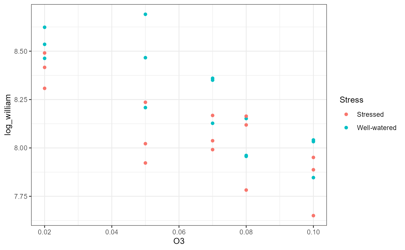

add a geom_smooth() layer
instead of using automatic calculations (method = "lm"), specify fit_data

ggplot(df,
       aes(x = O3, 
           y = log_william,
           color = Stress,
           fill = Stress)) +
  geom_point(size = 3) +
  theme_bw() +
  geom_smooth(data = fit_data,
              aes(y = fit, 
                  ymin = lwr, 
                  ymax = upr), 
                  stat = "identity")

ENVS475: Experimental Analysis and Design

Spring, 2023

About

ANCOVA

Preliminaries

Packages

Hypotheses, plain words

Hypotheses, graphs

Parameters, two linear equations

Data

Load data and rename object

Transform `William` variable

Plot data

Plot both predictor variables

Fit ANCOVA model

Assumptions

ANOVA table

Linear model summary

Equation for line 1: `Stressed`

Equation for line 2: `Well-watered`

Coda

Appendix: Plotting model estimates

Lab 14: ANCOVA

ENVS475: Experimental Analysis and Design

Spring, 2023

About

ANCOVA

Preliminaries

Packages

Hypotheses, plain words

Hypotheses, graphs

Parameters, two linear equations

Data

Load data and rename object

Transform William variable

Plot data

Plot both predictor variables

Fit ANCOVA model

Assumptions

ANOVA table

Linear model summary

Equation for line 1: Stressed

Equation for line 2: Well-watered

Coda

Appendix: Plotting model estimates

Transform `William` variable

Equation for line 1: `Stressed`

Equation for line 2: `Well-watered`