Lab 02: Introduction to R

What is `R`?

R is a free, open-source programming language and software environment for statistical computing, bioinformatics, visualization and general computing.

It is based on an ever-expanding set of analytical packages that perform specific analytical, plotting, and other programming tasks.

Why `R`?

R is free(!), runs on pretty much every operating system, and has a huge user base.

The use of R also promotes open science, and is one of the many possible solutions which are needed to remedy the replication crisis (also sometimes called the reproducibility crisis). Indeed, it is somewhat surprising how lax many researchers and journals are in documenting the statistical analyses conducted in research. The use of R scripts and judicious commenting (see below) along with the publication of raw data will vastly improve scientific fields moving forward.

R is far from the only programming language for working with data. But it is the most widely used language in the fields of ecology, and environmental sciences. If you plan to pursue a career in any of these fields, proficiency in Ris quickly becoming a prerequisite for many jobs.

Even if you don’t pursue a career in one of these fields, the ability to manipulate, analyze, and visualize data (otherwise known as data science) is an extremely marketable skill in many professions right now.

Additional resources and where to get help

Cheat Sheets. In Rstudio, click Help > Cheat Sheets and select the appropriate one. The RStudio IDE is a good place to start. Even after nearly a decade of using R regularly, I often have the Data transformation with dplyr and Data visualization with ggplot2 when I’m doing almost anything in Rstudio. You can also Google “R Cheat Sheets” to find others which are available.

We will go over the basics of using R in class but there are many good online resources for learning R and getting help. A few of my favorites include:

Clark Rushing’s FANR6750 website (from which much of this material is borrowed)
Data Carpentry for Biologists (also from which much of this material is borrowed)
R for Data Science Which is a completely free book online and covers many of the important aspects of working in R.

Of course, if you encounter error messages you don’t understand or need help figuring out how to accomplish something in R, google is your best friend (even the most experienced R users use google on a daily basis, myself included). The key to finding answers on google is asking the right questions. Please refer to these links for advice on formulating R-related questions:

How to ask for R help
Seeking help from Data Analysis and Visualization in R for Ecologists

Using `R`- the very basics

As a statistical programming tool, one thing R is very good at is doing math. So as a starting point, let’s treat R like a fancy calculator.

We interact with this calculator by typing numbers and operators (+, -, *, /) into the Console window. By default, the Console window is in the bottom left, but you can customize the display of windows in RStudio by clicking on Tools > Global Options > Pane Layout. For example, I like to have my Console window in the bottom right, and the Source window in the bottom left.

Basic expressions

Let’s try it - in the Console, write the R code required to add two plus two and then press enter:

2+2

When you run the code, you should see the answer printed below the window. Play with your code a bit - try changing the number and the operators and then run the code again. For example, try multiplying with *, division with /, and exponents with ^ or with **. Also, play around with order of operations and the use of () in your basic expressions.

Objects

Scalars

We can run R like a calculator by typing equations directly into the console and then printing the answer. But usually we don’t want to just do a calculation and see the answer. Instead, we assign values to objects. That object is then saved in R’s memory which allows us to use that object later in our analysis.

This might seem a bit confusing if you are new to programming so let’s try it. The following code creates an object called x and assigns it a value of 3:

x <- 3

The operator <- is how we do assignments in R. Whatever is to the left of <- is the object’s name and whatever is to the right is the value. As we will see later, objects can be much more complex than simply a number but for now, we’ll keep it simple.

RStudio has built in shorcuts for the <- operator: Alt + - (Windows) or Option + - (Mac).

Removing objects

If you no longer want an object to be in your working environment, you can use the rm() command. If you ran the x <- 3 command above, you should see an x object in your Environment panel. After you confirm that you have an x object there, run the following code:

rm(x)

After running this, the x object should no longer be in your Environment.

You try it - change the code to create an object called new_x. Instead of assigning new_x a number, give it a calculation, for example 25/5. What do you think the value of new_x is?

Working with objects

In the exercise above, you may have noticed that after running the code, R did not print anything. That is because we simply told R to create the object (if you click on the Environment tab, you should see x and new_x). Now that it is stored in R’s memory, we can do a lot of things with it. For one, we can print it to see the value. To do that, we simply type the name of the object and run the code:

new_x <- 25/5
new_x
#> [1] 5

We can also use objects to create new objects. What do you think the following code does?

x <- 3
y <- x * 4

After running it, print the new object y to see its value. Were you right?

We can do more complex manipulations and give our variables meaningful names. For example, perhaps we are doing surveys of nesting birds and want to get an estimate on the total weight of eggs in a nest. Let’s say we have 6 eggs in a nest, and each egg weighs an average of 14 grams. Note that the last line is the name of the object that we created. We include this line of code so that R sill tell us the value of that object.


n_eggs <- 6
egg_mass_g <- 14
egg_mass_total <- n_eggs * egg_mass_g
egg_mass_total
#> [1] 84

Naming objects

It’s a good idea to give objects names that tell you something about what the object represents. Names can be as long as you want them to be but can not have spaces.

Snake Case (my preferred method)

I prefer to use snake case where an underscore (_) is used to separate words in object names (for example: my_data_object, filtered_data, etc).

Other options

Other options include camelCase where no spaces or separators are used but new words are capitalized (for example: myDataObject, filteredData, etc.), or using . to separate words (my.data.object, filtered.data, etc.). I strongly recommend against using periods to separate words. In this class it most likely won’t come up, but R often uses . in internal functions, and as you advance in your programming abilities it may become an issue. Better to not make bad habits from the beginning then try to break them later.

Also remember long names require more typing so brevity is a good rule of thumb. Names also cannot start with a number and R is case-sensitive so, for example, Apple is not the same as apple.

Built-in functions

A function is a complicated expression.
Command that returns a value

sqrt(49)
#> [1] 7

A function call is composed of two parts.
- Name of the function
- Arguments that the function requires to calculate the value it returns.
- sqrt() is the name of the function, and 49 is the argument.
We can also pass variables as the argument

weight_lb <- 0.11
sqrt(weight_lb)
#> [1] 0.3316625

Another function that we’ll use a lot is str()
All values and therefore all variables have types
str, short for “structure”, lets us look at them

str(weight_lb)
#>  num 0.11

Another data type is for text data, called “character”
We write text inside of quotation makes

"hello world"
#> [1] "hello world"

We can use the str() and class() functions to look at the “structure” and “class of the object

str("hello world")
#>  chr "hello world"
class("hello world")
#> [1] "character"

Function Arguments

Functions can take multiple arguments.
- The round() function is used to round numbers to a specific decimal point
- Type ?round in the console
- in the help window that pops up, scroll down to the Usage which shows there are two arguments:
  - x: Number to be rounded
  - digits: number of digits

round(x = weight_lb, digits = 1)
#> [1] 0.1

NOTE If you enter the arguments in the same order as they show up in the function you do not have to name them:

round(weight_lb, 1)
#> [1] 0.1

Although you don’t have to name arguments, it’s a good idea to get in the habit of naming them. This will make you code easier to read, will help avoid mistakes that can occur when you don’t put the arguments in the correct order, and makes it easier to trouble shoot code that doesn’t do what you expect it to do.

Likewise, if you name the arguments, you can put them in different order and it will still run correctly:

round(digits = 1, x = weight_lb)
#> [1] 0.1

You try it - modify the code above to round weight_lb to the 4th decimal point.

If you do name the arguments, you can switch their order:

round(digits = 0, x = y)
#> [1] 12

Functions return values, so as with other values and expressions, if we don’t save the output of a function then there is no way to access it later
It is common to forget this when dealing with functions and expect the function to have changed the value of the variable
But looking at weight_lb we see that it hasn’t been rounded

weight_lb
#> [1] 0.11

To save the output of a function we assign it to a variable.

weight_rounded <- round(weight_lb, digits = 1)
weight_rounded
#> [1] 0.1

Using scripts instead of the console

The console is useful for doing simple tasks but as our analyses become more complicated, the console is not very efficient. What if you need to go back and change a line of code? What if you want to show your code to someone else to get help?

Instead of using the console, most of our work will be done using scripts. Scripts are special files that us to write, save, and run many lines of code. Scripts can be saved so you can work on them later or send them to collaborators.

To create a script, click File -> New File -> R Script. You can also select the white square with a green plus sign on it in the top left of Rstudio and select the R Script option. Finally, if you don’t want to use your mouse or prefer keyboard shortcuts, you can also press Ctrl + Shift + N (windows) or Cmd + Shift + N (mac). This new file should show up in a new window.

Shortcuts

As you gain more coding experience, you may be interested in learning more shortcuts. A full list (Windows and Mac) can be found here

Commenting your code

R will ignore any code that follows a #. This is very useful for making your code more readable for both yourself and others. Use comments to remind yourself what a newly created object is, to explain what a line of code does, to leave yourself a reminder for later, etc. For example, let’s say you are working with mark-recapture data and you have the following code:

n1 <- 44     
n2 <- 32     
m2 <- 15

When you entered the code, you probably knew what each object name meant. But if you come back to it six months from now you might not have any idea what’s going on.

This is a great example of when to use comments to define what each object represents:

n1 <- 44     # Number of individuals captured on first occasion

n2 <- 32     # Number of individuals captured on second occasion
  
m2 <- 15     # Number of previously marked individuals captured on second occasion

Notice that when you run this code, R ignores the comments.

You can also put a commented line above the code you want to comment. This is my preferred method, and works better if you need a long comment.

If you need to put in a longer comment, you will need to put a # in front of every line. For example (don’t worry about the code for now, just observe the comments):

# load the pre-built data set in R called "CO2"

data(CO2)

# what are the names of the columns?
names(CO2)
#> [1] "Plant"     "Type"      "Treatment" "conc"      "uptake"

# we are only interested in the "chilled"  treatment group
# filter out this group and save in a new object for
# further analysis
# also switching to lower case for easier typing
co2_chilled <- CO2[CO2$Treatment == "chilled",]

# what is the average uptake of the chilled treatment?
mean(co2_chilled$uptake)
#> [1] 23.78333

You can run the entire script by selecting “source” at the top right of the script window (recommend selecting the down arrow and choosing “source with echo”). Likewise, you can run the entire script with echo with the shortcut Ctrl+Shift+Enter (windows) or Cmd+Shift+Return (mac).

You can also run individual lines of code in the script by putting your cursor on that line and pressing Ctrl+Enter (windows) or Cmd+Return (mac). When you do this, your cursor automatically moves to the next line. The line-by-line method is preferred when you are working out code or trying to figure out sections, problems, etc.

Vectors

So far, we have only been working with objects that store a single number (called scalars in programming jargon). However, often it is more convenient to store a string of numbers as a single object. In R, these strings are called vectors and they are usually created by enclosing the string between c( and ).

c() is for “concatenate” which means link things together in a chain or series:

x <- c(3,5,2,5)
x
#> [1] 3 5 2 5

You can also store sequences of consecutive numbers in a few different ways:

x <- 1:10
x
#>  [1]  1  2  3  4  5  6  7  8  9 10

x2 <- seq(from = 1, to = 10, by = 1)
x2
#>  [1]  1  2  3  4  5  6  7  8  9 10

Using Functions to make Vectors

A quick note on functions in R. We will be using functions heavily in this class. Functions take the form of function_name(), where the () enclose the function arguments. So in the call above: seq(from = 1, to = 10, by = 1) we are saying: produce a sequence of numbers from 1 (from = 1) to 10 (to = 10), and do it for each integer (by = 1). Note that you can enter the arguments without names if you put them in the correct order: seq(1, 10, 1). However, while learning I STRONGLY encourage you to write out the argument names. This will undoubtedly avoid lots of confusion and frustration.

The seq() function is very flexible and useful so if you are not familiar with it, be sure to look at the help page to better understand how to use it. for example, note the length.out argument. This can be useful if you want a vector of a certain length (i.e., number of values) between a minimum and maximum value, but aren’t sure what by = ? value to use. In this case, you would leave out the by = argument and only use the length.out = argument.

x3 <- seq(from = 1, to = 10, length.out = 5)
x3
#> [1]  1.00  3.25  5.50  7.75 10.00

You try it - change the seq() call to make a vector from 1 to 20 which has 8 values, and store it as x4.

Another useful function for creating vectors is rep(), which repeats values of a vector:

rep(x2, times = 2)
#>  [1]  1  2  3  4  5  6  7  8  9 10  1  2  3  4  5  6  7  8  9 10

or:

rep(x2, each = 2)
#>  [1]  1  1  2  2  3  3  4  4  5  5  6  6  7  7  8  8  9  9 10 10

Be sure you notice the difference between using the times argument vs the each argument!

Vectors: Numeric OR Character

A vector can also contain characters (though you cannot mix numbers and characters in the same vector!):

occasions <- c("Occasion1", "Occasion2", "Occasion3")
occasions
#> [1] "Occasion1" "Occasion2" "Occasion3"

The quotes around “Occasion1”, “Occasion2”, and “Occasion3” are critical. Without the quotes, R will assume there are objects called Occasion1, Occasion2 and Occasion3. As these objects don’t exist in R’s memory, there will be an error message.

You try it - modify the code above removing the " " around the different occassions within the c( ). What does the Error message tell you? ***

Vectors can be any length (including 1. In fact, the numeric objects we’ve been working with are just vectors with length 1). The function length() tells you how long a vector is:

# first, recall what the value of x is
x
#>  [1]  1  2  3  4  5  6  7  8  9 10
# what is the length of x?
length(x)
#> [1] 10

The function class() indicates the class (the type of element) of an object:

class(x)
#> [1] "integer"
class(occasions)
#> [1] "character"

What is the class of a vector with both numeric and characters entries? Hint:

mixed <- c(1, 2, "3", "4")

Print out the mixed object in the console. What does it look like? What happend to the numbers and the characters in the vector? You can also type class(mixed) to confirm what R “thinks” it is.

You can also use the c() function to add other elements to your vector:

# first, recall what value you stored in "x"
x
#>  [1]  1  2  3  4  5  6  7  8  9 10

# now make a new vector y, with x and other numbers
y <- c(x, 4, 8, 3)

Vectors are one of the many data structures that R uses. Other important ones are lists (list()), matrices (matrix()), data frames (data.frame()), factors (factor()) and arrays (array()). We will learn about each of those data structures as we encounter them in lab exercises.

Indexing vectors

Often you will need to work with just a subset of a vector. For example, maybe you have a vector of plant biomass measured along transects but you only need the third observation:

y <- c(2, 4, 8, 5, 25, 3, 6, 1)
y[3]
#> [1] 8

Notice that to index certain elements of the vector y, we use square brackets []. Inside those brackets, we provided an integer to refer to the position of elements in the vector. The indexing vector can be more than length = 1, but to do that we need to group them using the c() function. For example, let’s say we wanted the 1st and the 3rd observation in a vector:

y[c(1,3)]
#> [1] 2 8

You try it - subset the y vector to have the 1st and 3rd to 5th, and 8th observation ***

We can also index vectors using a logical vector. A logical vector is a special type of object that contains values of TRUE or FALSE. When using a logical vector for indexing, the logical vector indicates which elements to keep (TRUE) or remove (FALSE) from the original vector. For this reason, the indexing vector must be same length as the focal vector; i.e., length(a) == length(v)

# Logical vector (which elements of y are greater than 4?)
y > 5
#> [1] FALSE FALSE  TRUE FALSE  TRUE FALSE  TRUE FALSE

# Indexing using a logical vector (keep elements 3, 5 and 7)
y[y > 5]
#> [1]  8 25  6

We can also use indexing to remove elements from a vector:

# Remove the second element
y[-2]
#> [1]  2  8  5 25  3  6  1

or to rearrange the order of a vector

y[c(5,4,3,2,1)]
#> [1] 25  5  8  4  2

Functions on Vectors

More Built-in functions

The power of R is most apparent in the large number of built-in functions that are available for users.

Functions are small bits of code that perform a specific task. Most functions accept one or more inputs called arguments and return a value or a new object.

Let’s say we have the following data on the number of ticks recorded on 5 dogs:

Individual	Ticks
1	4
2	7
3	2
4	3
5	150

What is the total number of ticks recorded in the study? For that, we can use the built-in sum() function:

ticks <- c(4, 7, 2, 3, 150)

sum(ticks)
#> [1] 166

What is the mean number of ticks per dog?

mean(ticks)
#> [1] 33.2

And the variance?

var(ticks)
#> [1] 4266.7

We can also calculate common summary statistics
For example, if we have a vector of population counts

count <- c(9, 16, 3, 10)
mean(count)
#> [1] 9.5
max(count)
#> [1] 16
min(count)
#> [1] 3
sum(count)
#> [1] 38

`NULL`s in vectors

So far we’ve worked with vectors that contain no missing values
But most real world data has values that are missing for a variety of reasons
For example, kangaroo rats don’t like being caught by humans and are pretty good at escaping before you’ve finished measuring them
Missing values, known as “null” values, are written in R as NA with no quotes, which is short for “not available”
So a vector of 4 population counts with the third value missing would look like

count_na <- c(9, 16, NA, 10)

If we try to take the mean of this vector we get NA?

mean(count_na)
#> [1] NA

Hard to say what a calculation including NA should be
So most calculations return NA when NA is in the data
Can tell many functions to remove the NA before calculating
Do this using an optional argument, which is an argument that we don’t have to include unless we want to modify the default behavior of the function
Add optional arguments by providing their name (na.rm), =, and the value that we want those arguments to take (TRUE)

mean(count_na, na.rm = TRUE)
#> [1] 11.66667

Vectorized arithmetic

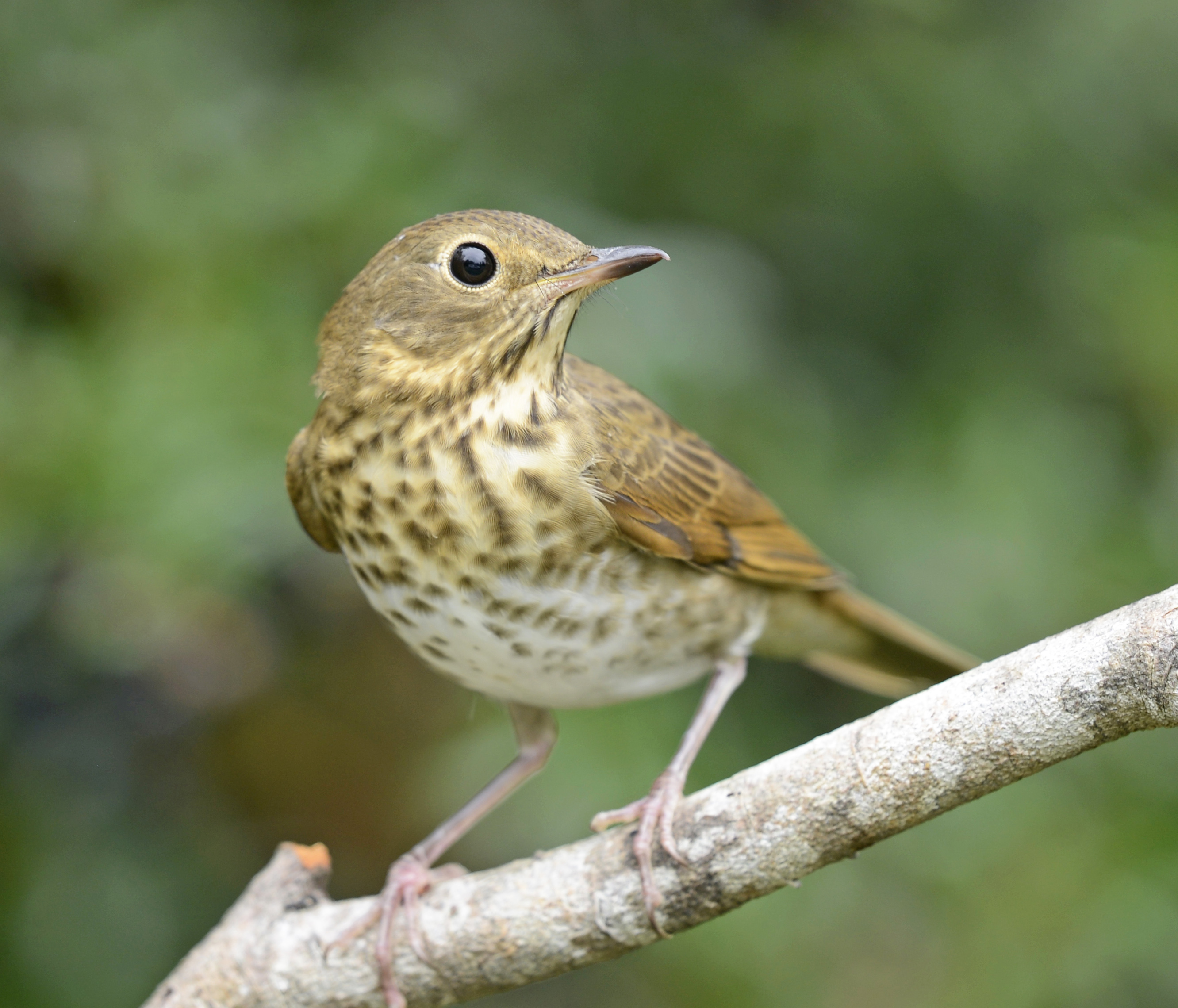
One of the most useful properties of vectors in R is that we can use them to simplify basic arithmetic operations that need to be done on multiple observations. For example, consider the following data on wing chord (a measure of wing length) and body mass of Swainson’s thrushes (Catharus ustulatus):

Swainson’s Thrush. Image courtesy of VJAnderson via Wikicommons

Image link

Individual	Mass (g)	Wing chord (mm)
1	36.2	95.1
2	34.6	88.4
3	31.0	97.9
4	31.8	96.8
5	29.4	92.3
6	32.0	90.6

Perhaps we want to derive the body condition of each individual based on these measures. One common metric of body condition used by ornithologists is $\frac{mass}{size}$, where wing chord is used as a proxy for body size. We could calculate body condition for each individual:

cond1 <- 36.2/95.1 # Body condition of the first individual

cond2 <- 34.6/88.4 # Body condition of the second individual

But that is time consuming and error prone. Luckily, R will vectorize basic arithmetic:

mass <- c(36.2, 34.6, 31.0, 31.8, 29.4, 32.0)
wing <- c(95.1, 88.4, 97.9, 96.8, 92.3, 90.6)

cond <- mass/wing
cond
#> [1] 0.3806519 0.3914027 0.3166496 0.3285124 0.3185265 0.3532009

As you can see, when we divide one vector by another, R divides the first element of the first vector by the first element of the second vector, etc. and returns a vector.

Packages

One of R’s primary strengths is the large number of packages available to users. Packages are units of shareable code and data that have been created by other R users. We have already seen the built-in functions that R comes with. Packages allow users to share lots and lots of other functions that serve specific purposes. Packages also allow users to share data sets. There are packages for cleaning data, visualizing data, making maps, fitting specialized models, and basically anything else you can think of.

Accessing the code in a package first requires installing the package. This only needs to be done once per computer and is usually done using the install.packages() function:

install.packages("dplyr")

Note that the name of the package (in this case dplyr) must be in quotation marks. Packages installed using install.packages() are stored in a centralized repository called CRAN (Comprehensive R Archive Network). Once dplyr (or any package) is installed on your computer, you do not need to re-run the install.packages() function unless you re-install/update R or need to update the package to a newer version.

dplyr is a powerful package for summarizing and modifying data which we will use extensively in class. We will have a more thorough introduction to dplyr later this semester.

Note if you will be using your own personal laptop for this course, you will only need to run the install.packages() function once. However, if you will be using the department laptops in class, and then a desktop computer at home or in the library, computer labs, etc., you will need to run install.packages() the first time you use each computer. Likewise, if you are using university computers in the library or computer labs, you may need to install.packages() each time you log on (it’s unclear if the University IT security procedures will remove these regularly or not).

Installing a package does not automatically make the functions from that package available in a given R session. To tell R where the functions come from, you must load the package using the library() function:

library(dplyr)

Unlike install.packages(), library() must be re-run each time you open R. Most people include a few calls to library() at the beginning of each script so that all packages needed to run the code are loaded at the beginning of the script.

Data frames

So far, we have only discussed one particular class of R object - vectors. Vectors hold a string of values as a single object. Although useful for many applications, vectors are limited in their ability to store multiple types of data (numeric and character).

This is where data frames become useful. Perhaps the most common type data object you will use in R is the data frame. Data frames are tabular objects (rows and columns) similar in structure to spreadsheets (think Excel or GoogleSheets). In effect, data frames store multiple vectors - each column of the data frame is a vector. As such, each column can be a different class (numeric, character, etc.) but all values within a column must be the same class. Just as the first row of an Excel spreadsheet can be a list of column names, each column in a data frame has a name that (hopefully) provides information about what the values in that column represent. The names of columns in data frames are often referred to as variables while the rows are generally referred to as observations.

To see how data frames work, let’s load a data frame called starwars that comes with the dplyr package.

library(dplyr)
# the data() function loads data sets which are built-in 
# or that come with packages
data("starwars")

If you ran the library(dplyr) function above, you do not strictly need to run it here again, but i included it here to ensure that you have this package loaded. The data() function access the built-in data set called "starwars" and makes it accessible in your working session. After running that call, you should see a starwars data object in your Environment tab.

Note - As discussed above, if you want to access function or data sets that come with packages, you first need to load the package in your current working environment. To do that, use the library() function, with the unquoted package name as the argument. Once loaded, all of the package’s functions and built-in data sets are available to use.

Alternatively, you can access functions from a given package without loading the package using package.name::function.name(). For example, if you want to use the filter() function from the dplyr package, you could type dplyr::filter(). Although less commonly used, this method has a few advantages:

Sometimes different packages have functions with the same names. R will default to using the function from the package that was loaded last. For example, the raster package also has a function called filter() so if you load dplyr first (using library()and then raster, R will default to using raster’s filter() function, which could cause problems.
If you share your code with others, the :: method makes it clear which packages are being use for which functions. That additional clarity is often helpful and is the reason I will occasionally use :: in this course.

To get a quick idea of what information the starwars data frame contains, we can use the names() function, which returns the names of the columns, and the head() and tail() functions, which will print the first and last 6 rows of the data frame:

names(starwars)
#>  [1] "name"       "height"     "mass"       "hair_color" "skin_color"
#>  [6] "eye_color"  "birth_year" "sex"        "gender"     "homeworld" 
#> [11] "species"    "films"      "vehicles"   "starships"
head(starwars)
#> # A tibble: 6 × 14
#>   name      height  mass hair_color skin_color eye_color birth_year sex   gender
#>   <chr>      <int> <dbl> <chr>      <chr>      <chr>          <dbl> <chr> <chr> 
#> 1 Luke Sky…    172    77 blond      fair       blue            19   male  mascu…
#> 2 C-3PO        167    75 NA         gold       yellow         112   none  mascu…
#> 3 R2-D2         96    32 NA         white, bl… red             33   none  mascu…
#> 4 Darth Va…    202   136 none       white      yellow          41.9 male  mascu…
#> 5 Leia Org…    150    49 brown      light      brown           19   fema… femin…
#> 6 Owen Lars    178   120 brown, gr… light      blue            52   male  mascu…
#> # ℹ 5 more variables: homeworld <chr>, species <chr>, films <list>,
#> #   vehicles <list>, starships <list>
tail(starwars)
#> # A tibble: 6 × 14
#>   name      height  mass hair_color skin_color eye_color birth_year sex   gender
#>   <chr>      <int> <dbl> <chr>      <chr>      <chr>          <dbl> <chr> <chr> 
#> 1 Tion Med…    206    80 none       grey       black             NA male  mascu…
#> 2 Finn          NA    NA black      dark       dark              NA male  mascu…
#> 3 Rey           NA    NA brown      light      hazel             NA fema… femin…
#> 4 Poe Dame…     NA    NA brown      light      brown             NA male  mascu…
#> 5 BB8           NA    NA none       none       black             NA none  mascu…
#> 6 Captain …     NA    NA none       none       unknown           NA fema… femin…
#> # ℹ 5 more variables: homeworld <chr>, species <chr>, films <list>,
#> #   vehicles <list>, starships <list>

names() just tells us the names of the columns (aka variables) in the data frame. We also get this information from some of the other functions, but it is often helpful to get a reminder on the column names, and the output from names() is easier to interpret quickly.

We can see that starwars contains 14 columns with information on different characters in the star wars universe. The head() and tail() functions abbreviated the data presentation and only show the columns that easily fit on your screen. This is because the starwars object is a special kind of data.frame called a “tibble”.

class(starwars)
#> [1] "tbl_df"     "tbl"        "data.frame"

If we converted it to be just a data frame, it will show the first rows for all the columns:

head(as.data.frame(starwars))
#>             name height mass  hair_color  skin_color eye_color birth_year
#> 1 Luke Skywalker    172   77       blond        fair      blue       19.0
#> 2          C-3PO    167   75        <NA>        gold    yellow      112.0
#> 3          R2-D2     96   32        <NA> white, blue       red       33.0
#> 4    Darth Vader    202  136        none       white    yellow       41.9
#> 5    Leia Organa    150   49       brown       light     brown       19.0
#> 6      Owen Lars    178  120 brown, grey       light      blue       52.0
#>      sex    gender homeworld species
#> 1   male masculine  Tatooine   Human
#> 2   none masculine  Tatooine   Droid
#> 3   none masculine     Naboo   Droid
#> 4   male masculine  Tatooine   Human
#> 5 female  feminine  Alderaan   Human
#> 6   male masculine  Tatooine   Human
#>                                                                                                                                       films
#> 1                                           A New Hope, The Empire Strikes Back, Return of the Jedi, Revenge of the Sith, The Force Awakens
#> 2                    A New Hope, The Empire Strikes Back, Return of the Jedi, The Phantom Menace, Attack of the Clones, Revenge of the Sith
#> 3 A New Hope, The Empire Strikes Back, Return of the Jedi, The Phantom Menace, Attack of the Clones, Revenge of the Sith, The Force Awakens
#> 4                                                              A New Hope, The Empire Strikes Back, Return of the Jedi, Revenge of the Sith
#> 5                                           A New Hope, The Empire Strikes Back, Return of the Jedi, Revenge of the Sith, The Force Awakens
#> 6                                                                                     A New Hope, Attack of the Clones, Revenge of the Sith
#>                             vehicles                starships
#> 1 Snowspeeder, Imperial Speeder Bike X-wing, Imperial shuttle
#> 2                                                            
#> 3                                                            
#> 4                                             TIE Advanced x1
#> 5              Imperial Speeder Bike                         
#> 6

Several other useful functions exist for investigating the structure of data frames such as str() and summary(). I have not included the output of these in the tutorial, but you should run them to see what values they return.

str() tells us about the structure of the data frame, for example which columns are numeric or character class. summary() provides some simple summary statistics for each variable.

Other useful functions are dim(), nrow() and ncol(), which tells us the dimensions (number of rows and columns, in that order) number of columns, and how many rows are in the data frame (similar to length() for vectors):

dim(starwars)
#> [1] 87 14
nrow(starwars)
#> [1] 87
ncol(starwars)
#> [1] 14

Subsetting data frames

As you will see shortly, one of the most common tasks when working with data frames is creating new objects from parts of the full data frame. This task involves subsetting the data frame - selecting specific rows and columns. There are many ways of subsetting data frames in R, too many to discuss so we will only learn about a few.

Selecting columns

First, we may want to select a subset of all of the columns in a big data frame. Data frames are essentially tables, which means we can reference both rows and columns by their number: data.frame[row#, column#]. Note that you don’t actually type “row#”, you just enter the numer you want. for example, if you want the observation in the 1st row and the first column you would type:

starwars[1,1]
#> # A tibble: 1 × 1
#>   name          
#>   <chr>         
#> 1 Luke Skywalker

The row and column numbers have to put inside of square brackets following the name of the data frame object. The row number always comes first and the column number second. If you want to select all rows of a specific column, you just leave the row# blank. For example, if we wanted a vector containing just the home worlds (the 10th column) of all the characters:

starwars[,10]
#> # A tibble: 87 × 1
#>    homeworld
#>    <chr>    
#>  1 Tatooine 
#>  2 Tatooine 
#>  3 Naboo    
#>  4 Tatooine 
#>  5 Alderaan 
#>  6 Tatooine 
#>  7 Tatooine 
#>  8 Tatooine 
#>  9 Tatooine 
#> 10 Stewjon  
#> # ℹ 77 more rows

We can also select columns using data.frame$column_name (where data.frame is the name of the data frame object and column_name is the name of the column). In this case, you do actually need to type the $. For example,

starwars$homeworld
#>  [1] "Tatooine"       "Tatooine"       "Naboo"          "Tatooine"      
#>  [5] "Alderaan"       "Tatooine"       "Tatooine"       "Tatooine"      
#>  [9] "Tatooine"       "Stewjon"        "Tatooine"       "Eriadu"        
#> [13] "Kashyyyk"       "Corellia"       "Rodia"          "Nal Hutta"     
#> [17] "Corellia"       "Bestine IV"     NA               "Naboo"         
#> [21] "Kamino"         NA               "Trandosha"      "Socorro"       
#> [25] "Bespin"         "Mon Cala"       "Chandrila"      NA              
#> [29] "Endor"          "Sullust"        NA               "Cato Neimoidia"
#> [33] "Coruscant"      "Naboo"          "Naboo"          "Naboo"         
#> [37] "Naboo"          "Naboo"          "Toydaria"       "Malastare"     
#> [41] "Naboo"          "Tatooine"       "Dathomir"       "Ryloth"        
#> [45] "Ryloth"         "Aleen Minor"    "Vulpter"        "Troiken"       
#> [49] "Tund"           "Haruun Kal"     "Cerea"          "Glee Anselm"   
#> [53] "Iridonia"       "Coruscant"      "Iktotch"        "Quermia"       
#> [57] "Dorin"          "Champala"       "Naboo"          "Naboo"         
#> [61] "Tatooine"       "Geonosis"       "Mirial"         "Mirial"        
#> [65] "Naboo"          "Serenno"        "Alderaan"       "Concord Dawn"  
#> [69] "Zolan"          "Ojom"           "Kamino"         "Kamino"        
#> [73] "Coruscant"      NA               "Skako"          "Muunilinst"    
#> [77] "Shili"          "Kalee"          "Kashyyyk"       "Alderaan"      
#> [81] "Umbara"         "Utapau"         NA               NA              
#> [85] NA               NA               NA

Notice that if you hit tab after you type the $, RStudio will bring up all of the column names in that dataframe and you can use the up or down buttons to find the one you want.

Sometimes you may want to select more than one column. The easiest way to do that is to use the select() function in the dplyr package. Remember to run install.packages("dplyr") before the library(dplyr) call below if this is you’re first time using the dplyr package on the computer you are using.

library(dplyr)

head(select(.data = starwars, name, height, homeworld))
#> # A tibble: 6 × 3
#>   name           height homeworld
#>   <chr>           <int> <chr>    
#> 1 Luke Skywalker    172 Tatooine 
#> 2 C-3PO             167 Tatooine 
#> 3 R2-D2              96 Naboo    
#> 4 Darth Vader       202 Tatooine 
#> 5 Leia Organa       150 Alderaan 
#> 6 Owen Lars         178 Tatooine

Quick note I used the head() function around the select() function above to shorten the display of the starwars to save room. Nesting functions like this (head(select(...))) can be very useful. However, it can also be confusing because you have to read the functions “inside out”. Likewise it can be easy to miss or add additional () or , to either the beginning or the end of the function call. To help reduce this risk, I recommend turning on “rainbow brackets”: 1. Open Global Options from the Tools menu 2. Select Code -> Display 3. Enable the Rainbow Parentheses option at the bottom

Back to the select() function…

Notice that select requires us to first provide the data frame object (.data = starwars) and then we provide the column names (unquoted!) we want to select. You can also use select to remove columns:

head(select(.data = starwars, -height))
#> # A tibble: 6 × 13
#>   name    mass hair_color skin_color eye_color birth_year sex   gender homeworld
#>   <chr>  <dbl> <chr>      <chr>      <chr>          <dbl> <chr> <chr>  <chr>    
#> 1 Luke …    77 blond      fair       blue            19   male  mascu… Tatooine 
#> 2 C-3PO     75 NA         gold       yellow         112   none  mascu… Tatooine 
#> 3 R2-D2     32 NA         white, bl… red             33   none  mascu… Naboo    
#> 4 Darth…   136 none       white      yellow          41.9 male  mascu… Tatooine 
#> 5 Leia …    49 brown      light      brown           19   fema… femin… Alderaan 
#> 6 Owen …   120 brown, gr… light      blue            52   male  mascu… Tatooine 
#> # ℹ 4 more variables: species <chr>, films <list>, vehicles <list>,
#> #   starships <list>

You can also select all the columns that occur between two names using the :

head(select(.data = starwars, name:eye_color))
#> # A tibble: 6 × 6
#>   name           height  mass hair_color  skin_color  eye_color
#>   <chr>           <int> <dbl> <chr>       <chr>       <chr>    
#> 1 Luke Skywalker    172    77 blond       fair        blue     
#> 2 C-3PO             167    75 NA          gold        yellow   
#> 3 R2-D2              96    32 NA          white, blue red      
#> 4 Darth Vader       202   136 none        white       yellow   
#> 5 Leia Organa       150    49 brown       light       brown    
#> 6 Owen Lars         178   120 brown, grey light       blue

It’s important to realize that even though there are different ways to accomplish the same general task (in this case, “subset columns of a data frame”), those methods will sometimes differ in subtle but important ways.

For example, what type of object did the data.frame[,col#] and data.frame$column.name options return? What type of object did select(data.frame, col1, col2) return? Modify the code above by nesting it into the class() function to see what type of objects they are.

For example:

class(starwars$homeworld)
#> [1] "character"
class(select(.data = starwars, -height))
#> [1] "tbl_df"     "tbl"        "data.frame"

Those are very different results and knowing what the output will be can be useful when deciding the best way to accomplish your task i.e. if you want to have a vector or data.frame at the end.

Filtering rows

To select specific rows, we can use the [row#, col#] method we learned above, this time leaving the columns blank:

starwars[1,]
#> # A tibble: 1 × 14
#>   name      height  mass hair_color skin_color eye_color birth_year sex   gender
#>   <chr>      <int> <dbl> <chr>      <chr>      <chr>          <dbl> <chr> <chr> 
#> 1 Luke Sky…    172    77 blond      fair       blue              19 male  mascu…
#> # ℹ 5 more variables: homeworld <chr>, species <chr>, films <list>,
#> #   vehicles <list>, starships <list>

If we want more than one row, we just put in a vector with all of the rows we want:

# rows 1 and 2
starwars[1:2,]
#> # A tibble: 2 × 14
#>   name      height  mass hair_color skin_color eye_color birth_year sex   gender
#>   <chr>      <int> <dbl> <chr>      <chr>      <chr>          <dbl> <chr> <chr> 
#> 1 Luke Sky…    172    77 blond      fair       blue              19 male  mascu…
#> 2 C-3PO        167    75 NA         gold       yellow           112 none  mascu…
#> # ℹ 5 more variables: homeworld <chr>, species <chr>, films <list>,
#> #   vehicles <list>, starships <list>

# rows 1 and 30
starwars[c(1,30),]
#> # A tibble: 2 × 14
#>   name      height  mass hair_color skin_color eye_color birth_year sex   gender
#>   <chr>      <int> <dbl> <chr>      <chr>      <chr>          <dbl> <chr> <chr> 
#> 1 Luke Sky…    172    77 blond      fair       blue              19 male  mascu…
#> 2 Nien Nunb    160    68 none       grey       black             NA male  mascu…
#> # ℹ 5 more variables: homeworld <chr>, species <chr>, films <list>,
#> #   vehicles <list>, starships <list>

Note that we can use the square brackets to also subset vectors, in which case we don’t need the comma as long as you tell R which column you want first:

starwars$name[1]
#> [1] "Luke Skywalker"

Sometimes, we may not know the specific row number(s) we want but we do know the value of one of the columns we want to keep. Using the filter() function in the dplyr package allows us to filter rows based on the value of one of the variables. For example, if we want just characters from Tatooine, we use:

head(filter(starwars, homeworld == "Tatooine"))
#> # A tibble: 6 × 14
#>   name      height  mass hair_color skin_color eye_color birth_year sex   gender
#>   <chr>      <int> <dbl> <chr>      <chr>      <chr>          <dbl> <chr> <chr> 
#> 1 Luke Sky…    172    77 blond      fair       blue            19   male  mascu…
#> 2 C-3PO        167    75 NA         gold       yellow         112   none  mascu…
#> 3 Darth Va…    202   136 none       white      yellow          41.9 male  mascu…
#> 4 Owen Lars    178   120 brown, gr… light      blue            52   male  mascu…
#> 5 Beru Whi…    165    75 brown      light      blue            47   fema… femin…
#> 6 R5-D4         97    32 NA         white, red red             NA   none  mascu…
#> # ℹ 5 more variables: homeworld <chr>, species <chr>, films <list>,
#> #   vehicles <list>, starships <list>

Notice the need for two equals signs (==) when telling R we want the row where homeworld is Tatooine. A related task might be to filter out all the rows that are not Tatooine. In this case we would use the != operator which can be read “is not equal to”:

head(filter(starwars, homeworld != "Tatooine"))
#> # A tibble: 6 × 14
#>   name      height  mass hair_color skin_color eye_color birth_year sex   gender
#>   <chr>      <int> <dbl> <chr>      <chr>      <chr>          <dbl> <chr> <chr> 
#> 1 R2-D2         96    32 NA         white, bl… red               33 none  mascu…
#> 2 Leia Org…    150    49 brown      light      brown             19 fema… femin…
#> 3 Obi-Wan …    182    77 auburn, w… fair       blue-gray         57 male  mascu…
#> 4 Wilhuff …    180    NA auburn, g… fair       blue              64 male  mascu…
#> 5 Chewbacca    228   112 brown      unknown    blue             200 male  mascu…
#> 6 Han Solo     180    80 brown      fair       brown             29 male  mascu…
#> # ℹ 5 more variables: homeworld <chr>, species <chr>, films <list>,
#> #   vehicles <list>, starships <list>

Filter makes it very easy to select multiple rows using operators like greater than, less than, etc.

head(filter(starwars, height > 200))
#> # A tibble: 6 × 14
#>   name      height  mass hair_color skin_color eye_color birth_year sex   gender
#>   <chr>      <int> <dbl> <chr>      <chr>      <chr>          <dbl> <chr> <chr> 
#> 1 Darth Va…    202   136 none       white      yellow          41.9 male  mascu…
#> 2 Chewbacca    228   112 brown      unknown    blue           200   male  mascu…
#> 3 Roos Tar…    224    82 none       grey       orange          NA   male  mascu…
#> 4 Rugor Na…    206    NA none       green      orange          NA   male  mascu…
#> 5 Yarael P…    264    NA none       white      yellow          NA   male  mascu…
#> 6 Lama Su      229    88 none       grey       black           NA   male  mascu…
#> # ℹ 5 more variables: homeworld <chr>, species <chr>, films <list>,
#> #   vehicles <list>, starships <list>

It is also possible to use the “or” operator (|) when we want to select observations which meet different values. For example, we want observations of less than 80 OR > 200:

head(filter(starwars, height < 80 | height > 200))
#> # A tibble: 6 × 14
#>   name      height  mass hair_color skin_color eye_color birth_year sex   gender
#>   <chr>      <int> <dbl> <chr>      <chr>      <chr>          <dbl> <chr> <chr> 
#> 1 Darth Va…    202   136 none       white      yellow          41.9 male  mascu…
#> 2 Chewbacca    228   112 brown      unknown    blue           200   male  mascu…
#> 3 Yoda          66    17 white      green      brown          896   male  mascu…
#> 4 Roos Tar…    224    82 none       grey       orange          NA   male  mascu…
#> 5 Rugor Na…    206    NA none       green      orange          NA   male  mascu…
#> 6 Ratts Ty…     79    15 none       grey, blue unknown         NA   male  mascu…
#> # ℹ 5 more variables: homeworld <chr>, species <chr>, films <list>,
#> #   vehicles <list>, starships <list>

We can also filter out observations based on multiple columns using the “and” (&) operator. For example, we want the rows which have an height greater than 200, AND are from Tatooine:

head(filter(starwars, height > 200 & homeworld == "Tatooine"))
#> # A tibble: 1 × 14
#>   name      height  mass hair_color skin_color eye_color birth_year sex   gender
#>   <chr>      <int> <dbl> <chr>      <chr>      <chr>          <dbl> <chr> <chr> 
#> 1 Darth Va…    202   136 none       white      yellow          41.9 male  mascu…
#> # ℹ 5 more variables: homeworld <chr>, species <chr>, films <list>,
#> #   vehicles <list>, starships <list>

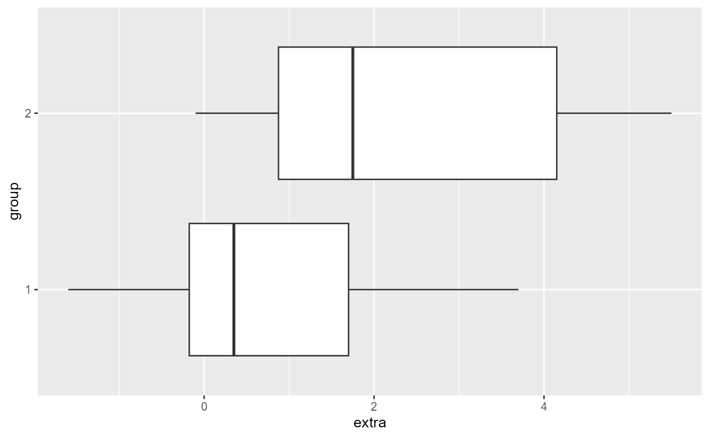
Assignment Formats: R Scripts

For your assignments, you will be writing R scripts with comments and code which solve problems and answer questions. You will submit your R scripts on D2L. I will download all the scripts and run them in RStudio on my computer to check your work. Therefore, you will need to follow strict assignment formatting rules.

File Names

Each assignment should follow this naming convention:

full_name_hwXX

For example: justin_pomeranz_hw01

You can capitalize words in the file name if you choose, but it should follow the general convention above.

File format

Comment before each problem, and each sub-problem
Make sure your results print out on Source with echo
- If you’re answer is saved in an object, make sure you print out that object afterwars
- for example, see the volume as the last line of the example below

# Problem 1

# 1.1
2+2

# 1.2
2 - 8

# problem 2

width = 2
height = 3
length = 1.5
volume = width * height * length
volume

Homework 1 - For a grade

Create an assignment script, put it in your class folder and name it according to the convention above.

We are going to get a feel for this by working through some exercises together.
In class we will often only do part of an exercise and save the rest for later or for you to do on your own.

See the homework 1 file for exercise descriptions.

ENVS475: Experimental Analysis and Design

Spring, 2023

What is `R`?

Why `R`?

Additional resources and where to get help

Using `R`- the very basics

Basic expressions

Objects

Scalars

Removing objects

Working with objects

Naming objects

Snake Case (my preferred method)

Other options

Built-in functions

Function Arguments

Using scripts instead of the console

Shortcuts

Commenting your code

Vectors

Using Functions to make Vectors

Vectors: Numeric OR Character

Indexing vectors

Functions on Vectors

More Built-in functions

`NULL`s in vectors

Vectorized arithmetic

Packages

Data frames

Subsetting data frames

Selecting columns

Filtering rows

Assignment Formats: R Scripts

File Names

File format

Homework 1 - For a grade

Lab 02: Introduction to R

ENVS475: Experimental Analysis and Design

Spring, 2023

What is R?

Why R?

Additional resources and where to get help

Using R- the very basics

Basic expressions

Objects

Scalars

Removing objects

Working with objects

Naming objects

Snake Case (my preferred method)

Other options

Built-in functions

Function Arguments

Using scripts instead of the console

Shortcuts

Commenting your code

Vectors

Using Functions to make Vectors

Vectors: Numeric OR Character

Indexing vectors

Functions on Vectors

More Built-in functions

NULLs in vectors

Vectorized arithmetic

Packages

Data frames

Subsetting data frames

Selecting columns

Filtering rows

Assignment Formats: R Scripts

File Names

File format

Homework 1 - For a grade

What is `R`?

Why `R`?

Using `R`- the very basics

`NULL`s in vectors