Lab 09: Tidy Data Entry

Overview

This week, we will discuss “tidy” data and how to enter data into spreadsheet software in a tidy format. This will help you get your own data into R in the future.

What is tidy data?

Each variable is a column; Each column is a variable
Each Observation is a row; Each row is an observation
Each value is a cell; Each cell is a value

Figure 1 shows these rules visually.

Three panels, each representing a tidy data frame. The first panel
shows that each variable is a column. The second panel shows that each
observation is a row. The third panel shows that each value is
a cell.

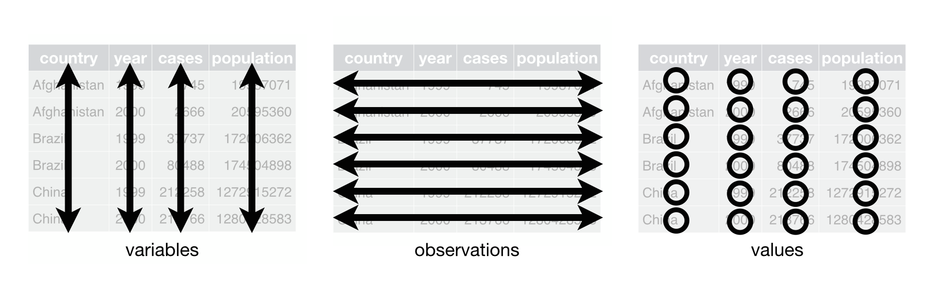
Figure 1. The following three rules make a dataset tidy: variables are columns, observations are rows, and values are cells. Fig from R4DS (2e), CC BY-NC-ND 3.0

Why use tidy data

One consistent way of storing data.

Easier to learn the tools
Underlying uniformity

Specific advantage to placing variables in columns

Allows R’s vectorized nature to shine.
most built-in R functions work with vectors of values.
That makes transforming tidy data feel particularly natural.
tidyverse
- Designed to work with tidy data.

Working with Tidy data

table1 is a small, tidy version of Tuberculosis infection data through time and by country.
It is automatically loaded with the tidyverse

table1

## # A tibble: 6 × 4
##   country      year  cases population
##   <chr>       <dbl>  <dbl>      <dbl>
## 1 Afghanistan  1999    745   19987071
## 2 Afghanistan  2000   2666   20595360
## 3 Brazil       1999  37737  172006362
## 4 Brazil       2000  80488  174504898
## 5 China        1999 212258 1272915272
## 6 China        2000 213766 1280428583

Every column is one variable, and every variable is one column
- country, year, cases, population
Every row is one observation.
- row 1 is the observation of TB cases and total population for Afghanistan in 1999, etc.
Every cell is a single value.
Consistent data set up
Takes advantage of R’s vectorized functions
Calculate the infection rate per 1000 people:

table1 |>
  mutate(rate = cases / population * 10000)

## # A tibble: 6 × 5
##   country      year  cases population  rate
##   <chr>       <dbl>  <dbl>      <dbl> <dbl>
## 1 Afghanistan  1999    745   19987071 0.373
## 2 Afghanistan  2000   2666   20595360 1.29 
## 3 Brazil       1999  37737  172006362 2.19 
## 4 Brazil       2000  80488  174504898 4.61 
## 5 China        1999 212258 1272915272 1.67 
## 6 China        2000 213766 1280428583 1.67

It also allows for easy grouping
What is the total TB-infection numbers per year?

table1 |> 
  group_by(year) |> 
  summarize(total_cases = sum(cases))

## # A tibble: 2 × 2
##    year total_cases
##   <dbl>       <dbl>
## 1  1999      250740
## 2  2000      296920

And we can easily plug this into ggplot
Map aesthetics to variables.
- i.e., color = country

ggplot(table1, aes(x = year,
                   y = cases,
                   color = country)) +
  geom_line() +
  geom_point(size = 4) +
  theme_bw() +
  scale_x_continuous(breaks = c(1999, 2000))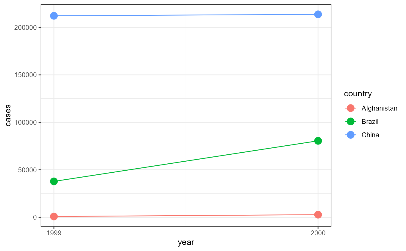

Long and Wide data

Data can be described as long (lots or rows)
or wide (lots of columns)
Generally, tidy data is “long”, but not always.
The tidyr package (part of the tidyverse) is made to make data tidy
pivot_longer() and pivot_wider() are the two primary functions
A full examination of tidyr is outside the scope of this course
- but if you’re interested, consider taking my intro to R course in the fall semester.

Untidy example

Long data, one column has many variables in it

table2 has the same data as table1 but it is in a long format

table2

## # A tibble: 12 × 4
##    country      year type            count
##    <chr>       <dbl> <chr>           <dbl>
##  1 Afghanistan  1999 cases             745
##  2 Afghanistan  1999 population   19987071
##  3 Afghanistan  2000 cases            2666
##  4 Afghanistan  2000 population   20595360
##  5 Brazil       1999 cases           37737
##  6 Brazil       1999 population  172006362
##  7 Brazil       2000 cases           80488
##  8 Brazil       2000 population  174504898
##  9 China        1999 cases          212258
## 10 China        1999 population 1272915272
## 11 China        2000 cases          213766
## 12 China        2000 population 1280428583

The problem here is that the type column actually has two variables in it:
- cases and population
To fix this data, we need to make two new columns called cases and population
We would remove the count column, and move the values into the appropriate new columns.
Here is an example of what the first two rows would look like.

tibble(country = "Afghanistan",
       year = 1999,
       cases = c(745, 2666),
       population = c(19987071, 20595360))

## # A tibble: 2 × 4
##   country      year cases population
##   <chr>       <dbl> <dbl>      <dbl>
## 1 Afghanistan  1999   745   19987071
## 2 Afghanistan  1999  2666   20595360

Variables in column names

Another common problem is that the columns have multiple variables in the names.
let’s look at a subset of the who2 data
- who2 is also a part of the tidyverse
- The who2 has TB data reported by country and year
- the column names has information on the:
  - Test type, i.e., sp, sn, ep
  - Patient sex: m or f
  - Patient age range 014, 1524…, 65

who2 |>
  select(country:sp_m_1524, sn_f_5564:sn_f_65) |>
  head()

## # A tibble: 6 × 6
##   country      year sp_m_014 sp_m_1524 sn_f_5564 sn_f_65
##   <chr>       <dbl>    <dbl>     <dbl>     <dbl>   <dbl>
## 1 Afghanistan  1980       NA        NA        NA      NA
## 2 Afghanistan  1981       NA        NA        NA      NA
## 3 Afghanistan  1982       NA        NA        NA      NA
## 4 Afghanistan  1983       NA        NA        NA      NA
## 5 Afghanistan  1984       NA        NA        NA      NA
## 6 Afghanistan  1985       NA        NA        NA      NA

This is a wide data format
In this example, the who2 data has 56 columns which could be presented in 3 columns (test type, sex, age range) and many more rows
In other words, this data needs to be transformed into a long format.

Your assignment will be to work on tidying a smaller version of this data

This concludes the lab

You should now begin your homework assignment

ENVS475: Experimental Analysis and Design