Lab 12: 2-Way ANOVA

About

This lab will demonstrate how to perform a two-way ANOVA with interaction in R. This includes checking assumptions, fitting the linear model, interpreting and visualizing the results.

Preliminaries

Packages

For this lab, we will be using the dplyr and ggplot2 packages. Make sure both packages are installed on your computer, and then run the following code:

library(tidyverse)

Data

We will use the ToothGrowth data which comes with R. Load the data by running the following command:

data("ToothGrowth")

ToothGrowth contains data examining the effect of varying the dose (dose) of two supplements (supp) on the length (len) of teeth in Guinea Pigs. Run ?ToothGrowth to learn more about the data.

Analysis

Let’s look at the full data, and see what the treatment levels are.

names(ToothGrowth)

## [1] "len"  "supp" "dose"

dim(ToothGrowth)

## [1] 60  3

head(ToothGrowth)

##    len supp dose
## 1  4.2   VC  0.5
## 2 11.5   VC  0.5
## 3  7.3   VC  0.5
## 4  5.8   VC  0.5
## 5  6.4   VC  0.5
## 6 10.0   VC  0.5

distinct(ToothGrowth, supp)

##   supp
## 1   VC
## 2   OJ

distinct(ToothGrowth, dose)

##   dose
## 1  0.5
## 2  1.0
## 3  2.0

distinct(ToothGrowth, supp, dose)

##   supp dose
## 1   VC  0.5
## 2   VC  1.0
## 3   VC  2.0
## 4   OJ  0.5
## 5   OJ  1.0
## 6   OJ  2.0

For this analysis, we have two factors (supp and dose). The supp factor has two levels: VC, and OJ and the dose factor has three levels: 0.5, 1.0, and 2.0.

Wrangle variables to be a Factor

You may have noticed that the dose variable is a class dbl. If we plug this into the lm() function, R will treat this as continuous and will give us a different result. In ANOVA, we want to analyze the data based on categories. We can chnage the dose variable to an ordered factor with the following code. We will also be changing the name of the data object to dat to have less typing to do.

dat <- ToothGrowth %>%
  mutate(dose = factor(dose,
                       levels = c(0.5, 1, 2),
                       labels = c("D0.5", "D1", "D2")))

We can also use the tab() function to see how many observations are in each group:

table(ToothGrowth$supp, ToothGrowth$dose)

##     
##      0.5  1  2
##   OJ  10 10 10
##   VC  10 10 10

We can see that there are 10 observations in each combination of all levels for both factors. We call this a completely balanced ANOVA design.

Plot data

Let’s start by plotting all of the data. We will save time and consider all the grouping variables.

ggplot(dat,
       aes(x = dose,
           y = len,
           color = supp)) +
  geom_boxplot() +
  theme_bw()

Interaction plots

We can estimate the effects based on the boxplot above, but an interaction plot is usually more illustrative.

Base R Plotting

with(data = dat, 
     interaction.plot(dose, supp, len))

`ggplot`

ggplot(dat, 
       aes(x = dose,
           y = len,
           color = supp,
           group = supp)) +
  geom_point() +
  stat_summary(fun = mean,
               geom = "line") +
  theme_bw()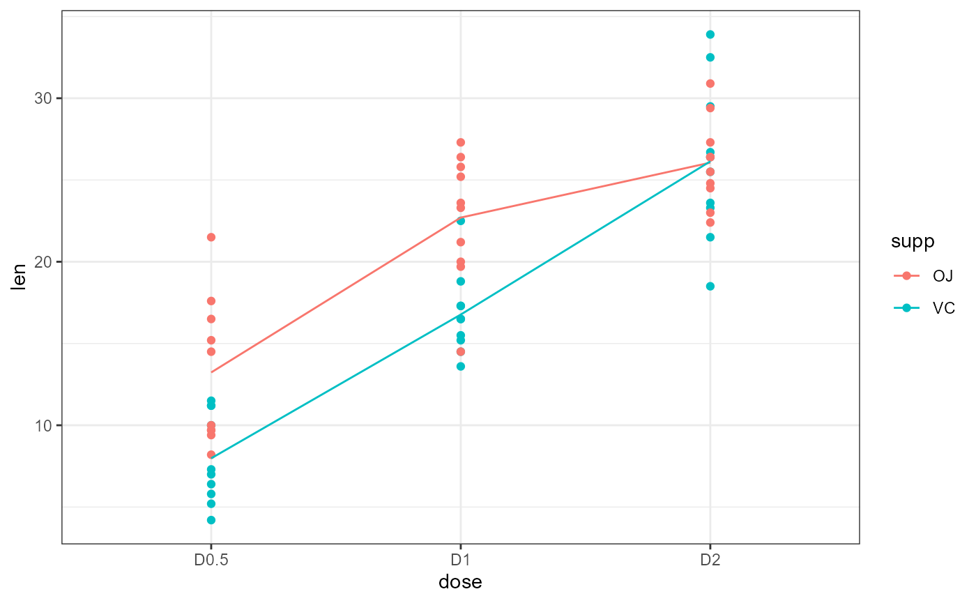

Check pre-analysis assumptions

Assumption: equal variance

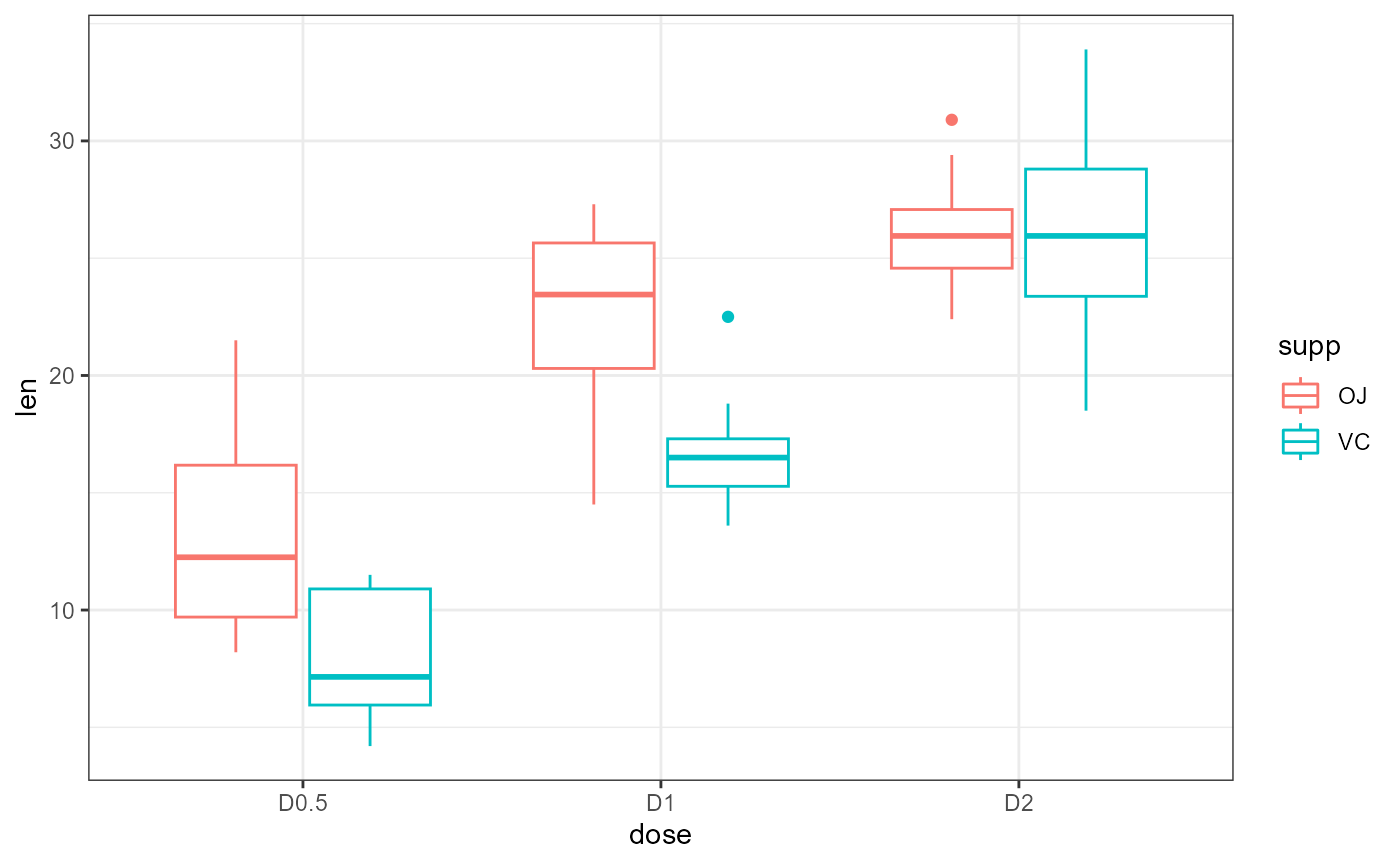
These data look to have approximately equal variation across the treatment groups. The D1:VC and D2:OJ look to have slightly less variation, but this is probably close enough.

Assumptions: Normality of residuals

QQ-plot

ggplot(dat,
       aes(sample = len)) +
  stat_qq()+
  stat_qq_line()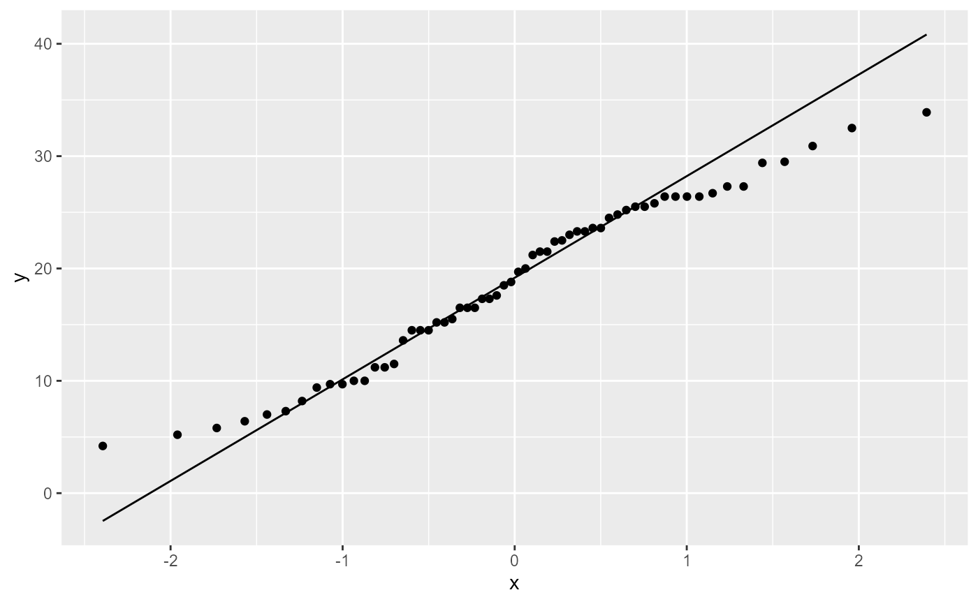

Most of the observations (points) fall close to the reference line. There’s a few that are off near the low and high end of the data, but this should be ok.

Two-way ANOVA

Hypotheses

Main effect of supplement (`supp`)

\[ H0: \text{There is NO effect of supplement on tooth growth} \]

\[HA: \text{There IS AN EFFECT of supplement on tooth growth}\]

Main effect of (`dose`)

Null and alternative hypotheses:

\[H0: \text{There is NO effect of Dose on tooth growth}\]

\[HA: \text{There IS AN EFFECT of Dose on tooth growth}\]

Interactive effect of `dose:supp`

\[H0: \text{The effect of one factor DOES NOT depend on the other factor}\] \[H0: \text{The effect of one factor DOES depend on the other factor}\]

Two-way ANOVA with `lm()`

Let’s first fit a linear model to the data.

tooth_lm <- lm(len ~ supp * dose, data = dat)
tooth_lm

## 
## Call:
## lm(formula = len ~ supp * dose, data = dat)
## 
## Coefficients:
##   (Intercept)         suppVC         doseD1         doseD2  suppVC:doseD1  
##         13.23          -5.25           9.47          12.83          -0.68  
## suppVC:doseD2  
##          5.33

Assumption: Equal variance of residuals

Before we look at the results, let’s check our post-model fit assumption with a fitted vs. residuals plot.

ggplot(tooth_lm,
       aes(x = .fitted, y = .resid)) +
    geom_point(
      position = position_jitter(
        width = 0.1,
        height = 0)) +
    geom_hline(yintercept = 0) +
  theme_bw()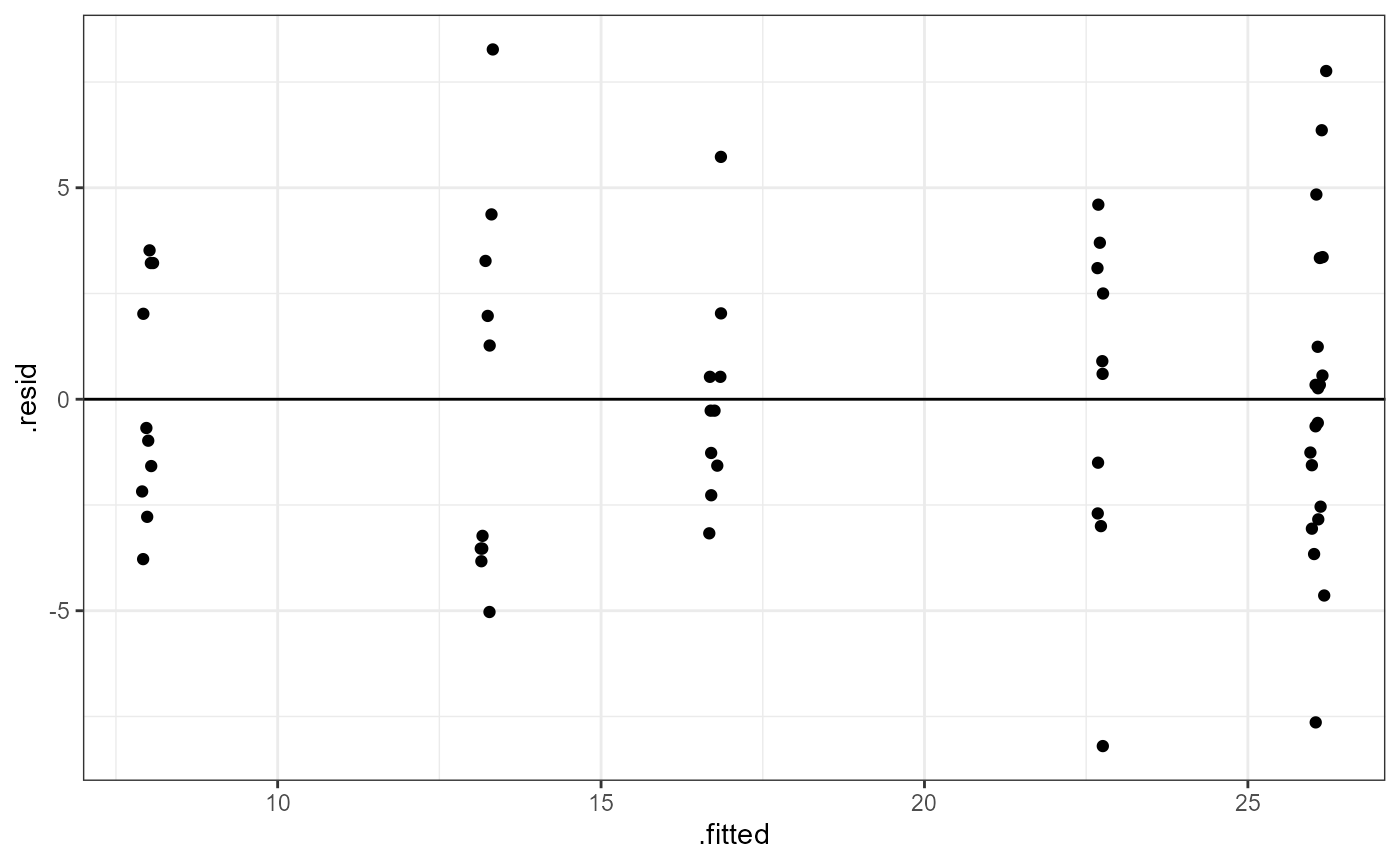

In this plot, the absolute magnitude of the maximum and minimum y-values are approximately the same (~ -7.5, ~ 7.5), although there are a couple of points above the 1.25 region. There may be slightly more variation on the right side (points are further from the line). However, there is no clear pattern in the spread of the points, so this looks OK.

ANOVA table

In order to get the statistical values for the ANOVA table, we need to use the anova() function on the model fit object.

anova(tooth_lm)

## Analysis of Variance Table
## 
## Response: len
##           Df  Sum Sq Mean Sq F value    Pr(>F)    
## supp       1  205.35  205.35  15.572 0.0002312 ***
## dose       2 2426.43 1213.22  92.000 < 2.2e-16 ***
## supp:dose  2  108.32   54.16   4.107 0.0218603 *  
## Residuals 54  712.11   13.19                      
## ---
## Signif. codes:  0 '***' 0.001 '**' 0.01 '*' 0.05 '.' 0.1 ' ' 1

You can see that we know have a row for each of the main factors and a row for the interaction effect (supp:dose) as well as a fourth row for the residuals (unexplained variation).

We interpret the F-value and p-value for each factor as before. Our interpretation of the main effects is the same as before. For example, there is a significant main effect of supplement (supp) and dose (dose).

We can now also make a statement of the statistical significance for the interactive effect. In this case, the p-value for the supp:dose interaction is p = 0.02 and this is less than our \(\alpha = 0.05\) cutoff, so there is an interactive effect. In other words, the effect of supplement depends on the dose applied (or the effect of the dose depends on the supplement type). Reminder do not try and interpret what the interaction effect is, just say that there is one.

ANOVA Interpretation

Remember that the hypotheses for ANOVA are either that all means are the same, or that at least one was different. ANOVA can only tell us that there is a difference. Therefore, our interpretation would look something like this:

Based on a 2-way ANOVA with interaction, there were significant main effects of supplement (\(F_{1, 54}= 15.572, p < 0.001\)) and dose (\(F_{2, 54}= 92, p < 0.001\)). Furthermore, there was a significnat interaction (\(F_{2, 54}= 4.1, p = 0.02\)) which means that the effect of one factor depended on the level of the other factor.

Relate ANOVA table to intercation plot

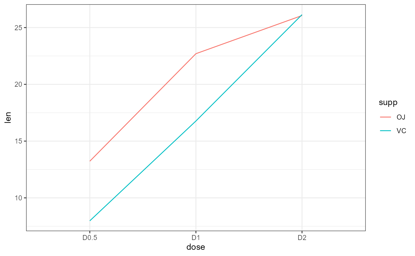
Main effect of `supp`

“Average” the y-values for each line individually across the x-values. Overall, the average of the red line is not equal to the average of the blue line: Significant main effect.

Main effect of `dose`

“Average” the y-values for each x-category across the lines. The average for D0.5 is low, and D1 is medium, while D2 is high. This means we have a significant effect of dose.

Interaction

Look at the lines to see if they are parallel or if they have a different slope. Both lines are parallel at the lower doses, but the slope changes between D1 and D2. This means there is a significant interaction.

Multiple Comparisons

In order to see which means are different, we can view the summary output from the lm() model, as well as calculate Tukey’s HSD.

`lm()` summary

summary(tooth_lm)

## 
## Call:
## lm(formula = len ~ supp * dose, data = dat)
## 
## Residuals:
##    Min     1Q Median     3Q    Max 
##  -8.20  -2.72  -0.27   2.65   8.27 
## 
## Coefficients:
##               Estimate Std. Error t value Pr(>|t|)    
## (Intercept)     13.230      1.148  11.521 3.60e-16 ***
## suppVC          -5.250      1.624  -3.233  0.00209 ** 
## doseD1           9.470      1.624   5.831 3.18e-07 ***
## doseD2          12.830      1.624   7.900 1.43e-10 ***
## suppVC:doseD1   -0.680      2.297  -0.296  0.76831    
## suppVC:doseD2    5.330      2.297   2.321  0.02411 *  
## ---
## Signif. codes:  0 '***' 0.001 '**' 0.01 '*' 0.05 '.' 0.1 ' ' 1
## 
## Residual standard error: 3.631 on 54 degrees of freedom
## Multiple R-squared:  0.7937, Adjusted R-squared:  0.7746 
## F-statistic: 41.56 on 5 and 54 DF,  p-value: < 2.2e-16

The summary output with multiple-levels of a factor and an interaction becomes much more complicated. However, if we take them one at-a-time we can see there’s not much different.

The intercept is the mean estimate for our reference group, which in this case is the OJ supplement at D0.5. We will need to keep this in mind when we look at all of the other coefficient estimates.

Other Coefficients:

suppVC = OJ:D0.5 - VC:D0.5
doseD1 = OJ:D0.5 - OJ:D1
doseD2 = OJ:D0.5 - OJ:D2
suppVC:doseD1 = OJ:D0.5 - VC:D1
suppVC:doseD2 = OJ:D0.5 - VC:D2

Interpretation of p-values

Intercept: Is mean length of OJ:D0.5 = 0?
- Low p-value, Reject null. Value is different from 0
Is the difference of the treatment group different from our reference group?
- reference group in this case is: OJ:D0.5
- suppVC:doseD1 has a high p-value, failt to reject (FTR) the null. In other words, it is not different from ’OJ:D0.5` (refer back to box plot)
- All other coefficients have p < 0.05, so reject the null hypothesis that those differences = 0. (In other words, there IS a difference between means.)

Tukey’s HSD

Before we run the Tukey HSD test, we need to run an ANOVA on our linear model fit using the aov() function.

# ANOVA of our lm model
tooth_aov <- aov(tooth_lm)

# Tukey's test on the plant_aov object
tooth_tukey <- TukeyHSD(tooth_aov)
# print out results
tooth_tukey

##   Tukey multiple comparisons of means
##     95% family-wise confidence level
## 
## Fit: aov(formula = tooth_lm)
## 
## $supp
##       diff       lwr       upr     p adj
## VC-OJ -3.7 -5.579828 -1.820172 0.0002312
## 
## $dose
##           diff       lwr       upr   p adj
## D1-D0.5  9.130  6.362488 11.897512 0.0e+00
## D2-D0.5 15.495 12.727488 18.262512 0.0e+00
## D2-D1    6.365  3.597488  9.132512 2.7e-06
## 
## $`supp:dose`
##                  diff        lwr        upr     p adj
## VC:D0.5-OJ:D0.5 -5.25 -10.048124 -0.4518762 0.0242521
## OJ:D1-OJ:D0.5    9.47   4.671876 14.2681238 0.0000046
## VC:D1-OJ:D0.5    3.54  -1.258124  8.3381238 0.2640208
## OJ:D2-OJ:D0.5   12.83   8.031876 17.6281238 0.0000000
## VC:D2-OJ:D0.5   12.91   8.111876 17.7081238 0.0000000
## OJ:D1-VC:D0.5   14.72   9.921876 19.5181238 0.0000000
## VC:D1-VC:D0.5    8.79   3.991876 13.5881238 0.0000210
## OJ:D2-VC:D0.5   18.08  13.281876 22.8781238 0.0000000
## VC:D2-VC:D0.5   18.16  13.361876 22.9581238 0.0000000
## VC:D1-OJ:D1     -5.93 -10.728124 -1.1318762 0.0073930
## OJ:D2-OJ:D1      3.36  -1.438124  8.1581238 0.3187361
## VC:D2-OJ:D1      3.44  -1.358124  8.2381238 0.2936430
## OJ:D2-VC:D1      9.29   4.491876 14.0881238 0.0000069
## VC:D2-VC:D1      9.37   4.571876 14.1681238 0.0000058
## VC:D2-OJ:D2      0.08  -4.718124  4.8781238 1.0000000

Here, we can see that we have a section for each factor as well as a section for the interaction. Witin each section there is a row for every pairwise combination. The table gives us an estimated and 95% CI for the differences, as well as an adjusted p value.

We can also plot these differences. Any coefficient estimates which cross zero are not considered to be significantly different.

plot(tooth_tukey)

Coda

This concludes Lab 12, and you should now be able to complete the homework assignment.

ENVS475: Experimental Analysis and Design

Spring, 2023

About

Preliminaries

Packages

Data

Analysis

Wrangle variables to be a Factor

Plot data

Interaction plots

Base R Plotting

`ggplot`

Check pre-analysis assumptions

Assumption: equal variance

Assumptions: Normality of residuals

QQ-plot

Two-way ANOVA

Hypotheses

Main effect of supplement (`supp`)

Main effect of (`dose`)

Interactive effect of `dose:supp`

Two-way ANOVA with `lm()`

Assumption: Equal variance of residuals

ANOVA table

ANOVA Interpretation

Relate ANOVA table to intercation plot

Main effect of `supp`

Main effect of `dose`

Interaction

Multiple Comparisons

`lm()` summary

Interpretation of p-values

Tukey’s HSD

Coda

Lab 12: 2-Way ANOVA

ENVS475: Experimental Analysis and Design

Spring, 2023

About

Preliminaries

Packages

Data

Analysis

Wrangle variables to be a Factor

Plot data

Interaction plots

Base R Plotting

ggplot

Check pre-analysis assumptions

Assumption: equal variance

Assumptions: Normality of residuals

QQ-plot

Two-way ANOVA

Hypotheses

Main effect of supplement (supp)

Main effect of (dose)

Interactive effect of dose:supp

Two-way ANOVA with lm()

Assumption: Equal variance of residuals

ANOVA table

ANOVA Interpretation

Relate ANOVA table to intercation plot

Main effect of supp

Main effect of dose

Interaction

Multiple Comparisons

lm() summary

Interpretation of p-values

Tukey’s HSD

Coda

`ggplot`

Main effect of supplement (`supp`)

Main effect of (`dose`)

Interactive effect of `dose:supp`

Two-way ANOVA with `lm()`

Main effect of `supp`

Main effect of `dose`

`lm()` summary