Learning Objectives
Following this assignment students should be able to:
- connect to a remote database and execute simple queries
- integrate database and R workflow
- export output data from R to database
- tidy data table with redundant fields or overfilled cells
Reading
-
Topics
RSQLitetidyr
-
Readings
- SQL databases and R
tidyrvignette- Optional Resources:
Lecture Notes
Exercises
Connect and Query
This is a follow up to the Basic Queries filtering problem.
It is clear Dr. Undómiel appreciates your skill working with large databases and she seems to expect you will maintain your benevolence. (Such is a fair expectation of a true wizard). This time though, she’s looking for some extra detail in her queries. She’s curious if desert rodents are dimorphic in size.
- Download a new copy of the Portal database.
- Connect to
portal_mammals.sqliteusing theRSQLitepackage. - Start by reminding yourself about which tables are in the database using
dbListTables() - Then remind yourself of the fields in the
surveysandplotstables usingdbListFields(). - Select and print out the average hind foot length and average weight of:
- all Dipodomys spectabilis individuals on the control plots
- male D. spectabilis on the control plots
- female D. spectabilis on the control plots
Automate Query
This is a follow-up to Connect and Query.
Dr. Undómiel agrees with you that the difference in male and female D. spectabilis hind foot length and weight seems pretty small, but wants to have a reference point for comparison. She wants you to find the male and female hind foot length and weight for all species of rodent on all of the plots (not just the controls).
Produce a data frame with
species_id,sex,avg_hindfoot_length, andavg_weightfor each species. Your data frame should have two rows for each species, one row for each sex.You can solve this problem in a variety of ways including using
Expected outputs for Automate Query: 1dplyr, aGROUP BYin your SQL query, aforloop, or usingapplystatements. Take whichever approach you like best.Export to Database
Dr. Undómiel has decided to focus on the change in size of a few target rodent species over the course of the experiment(1977-2002). She has chosen , Dipodymys spectabilis, Onychomys torridus, Perymiscus erimicus, Chaetodipus penicillatus.
Write a script that uses R and SQL to:
- Connect to the
portal_mammals.sqlite. - Generate a data frame with
year,species_id, and the average weight per year (avg_weight) for each target species. - Use
dbWriteTable()to include your new data frame in theportal_mammals.sqlite. Call it something informative so that Dr. Undómiel can find it easily.
- Connect to the
NEON Database
The National Ecological Observatory Network has entered into the construction phase of development and they are already making their data available! NEON collects ecological and environmental data for representative regions of the United States at local to continental scales, including, of course!, small mammal box trapping. We’ve retrieved NEON’s existing small mammal data from Ordway-Swisher Biological Station [NEON Data Use Policy].
- Create a SQLite database called
ordway_mammals.sqlite. - Download the three data tables (capture, plots, traps) and import them into the SQLite database.
- Connect to the database and familiarize yourself with its tables and structure.
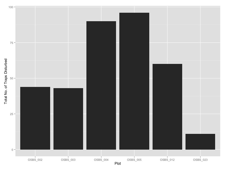
- Write a query to determine the total number of traps that have been disturbed at each plot. Plot a histogram of the results.
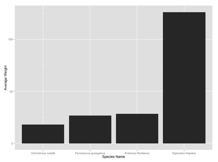
- Determine the average hind foot length and weight of each species collected
for each National Landcover Database (
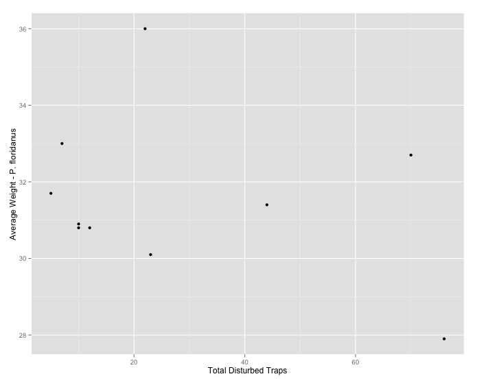
nlcd) class. Plot the average weight of all species with weight measurements from the woody wetlands. - Write a set of nested queries to determine the total number of disturbed traps and average weight of Podimus floridanus for each sampling event (
eventID).
- Create a SQLite database called
Tree Biomass
Estimating the total amount of biomass (the total mass of all individuals) in forests is important for understanding the global carbon budget and how the earth will respond to increases in carbon dioxide emissions. We can estimate the mass of a tree based on its diameter.
There are lots of equations for estimating the mass of a tree from its diameter, but one good option is the equation:
Mass = 0.124 * Diameter2.53
where
Massis measured in kg of dry above-ground biomass andDiameteris in cm DBH (Brown 1997).We’re going to estimate the total tree biomass for trees in a 96 hectare area of the Western Ghats in India. The data needs to be tidied before all of the tree stems can be used for analysis. f If the
Macroplot_data_Rev.txtis not already in your working directory download a copy.- Use
pivot_longer()to create a longer data frame with one row for each measured stem. Use dplyr’sfilterfunction to remove all of the girths that are zero. Store this longer data frame in a variable and also display it. - Write a function that takes a vector of tree diameters as an argument and
returns a vector of tree masses using the equation above. Test it usingmass_from_diameter(22). - Stems are measured in girth (i.e., circumference) rather than diameter.
Write a function that takes a vector of circumferences as an argument
and returns a vector of diameters (
diameter = circumference / pi). Test it usingdiameter_from_circumference(26). - Use the two functions you’ve written to and dplyr to add a
masscolumn to your longer data frame. Store this data in a variable and display it. - Estimate the total biomass by summing the mass of all of the stems in dataset.
separate()theSpCodecolumn intoGenusCodeandSpEpCodecolumns and then usegroup_byandsummarizeto the total biomass for each uniqueGenusCode.- Use ggplot to make a histogram of the
diametervalues. Make the x label"Diameter [cm]and the y label"Number of Stems"
- Use