Learning Objectives
The following assignment reviews:
- Basic translation between vector and data frame types
- Data wrangling pipelines using
dplyr- Basic
ggplot2functions
Reading
Lecture Notes
Exercises
Bird Banding Multiple Vectors (50 pts)
The number of birds banded at a series of sampling sites has been counted by your field crew and entered into the following vector. Counts are entered in order and sites are numbered starting at one. There is also information on the number of trees at each site. Cut and paste the vector into your assignment and then answer the following questions by using code and printing the result to the screen.
number_of_birds <- c(28, 32, 1, 0, 10, 22, 30, NA, 145, 27, 36, 25, 9, 38, 21, 12, 122, 87, 36, 3, 0, 5, 55, 62, 98, 32, 900, 33, 14, 39, 56, 81, 29, 38, 1, 0, 143, 37, 98, 77, 92, 83, 34, 98, 40, 45, 51, 17, 22, 37, 48, NA, 91, 73, 54, 46, 102, 273, 600, 10, 11) number_of_trees <- c(10, 12, 2, 3, 10, 8, 19, 19, 14, 3, 4, 5, 8, 4, 8, 1, 12, 10, 3, 1, 2, 3, 5, 6, 8, 2, 90, 3, 4, 3, 6, 8, NA, 4, 0, 1, 14, 3, 10, NA, 9, 8, 4, 8, 4, 4, 5, 1, 2, 3, 5, 4, 10, 7, 5, 8, 10, 30, 26, 1, 6)- How many sites are there?
- How many birds were counted at the 26th site?
- What is the largest number of birds counted?
- What is the average number of birds seen at a site?
- What is the total number of trees counted across all of the sites?
- What is the smallest number of trees counted?
- Produce a vector with the number of birds counted on sites with at least 10 trees.
- Produce a vector with the number of trees counted on sites with at least 10 trees.
- Combine the
number_of_birdsandnumber_of_treesvectors into a dataframe that also includes a year column with the year 2012 in every row and site column containing the numbers 1 through 61.
Portal Data Review (50 pts)
If
surveys.csv,species.csv, andplots.csvare not available in your workspace download them:Load them into R using
read.csv().- Create a data frame with only data for the
species_idDO, with the columnsyear,month,day,species_id, andweight. - Create a data frame with only data for species IDs
PPandPBand for years starting in 1995, with the columnsyear,species_id, andhindfoot_length, with no null values forhindfoot_length. - Create a data frame with the average
hindfoot_lengthfor eachspecies_idin eachyearwith no null values. - Create a data frame with the
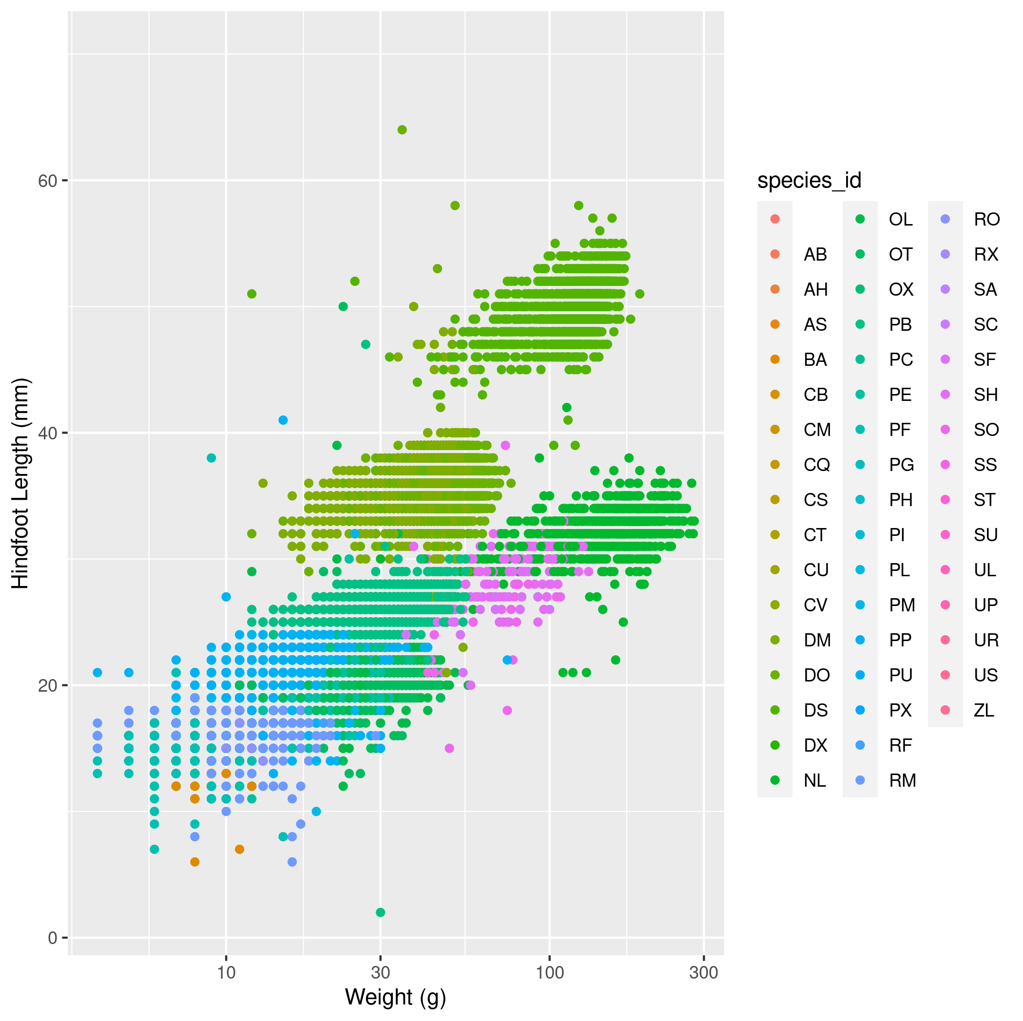
year,genus,species,weightandplot_typefor all cases where thegenusis"Dipodomys". - Make a scatter plot with
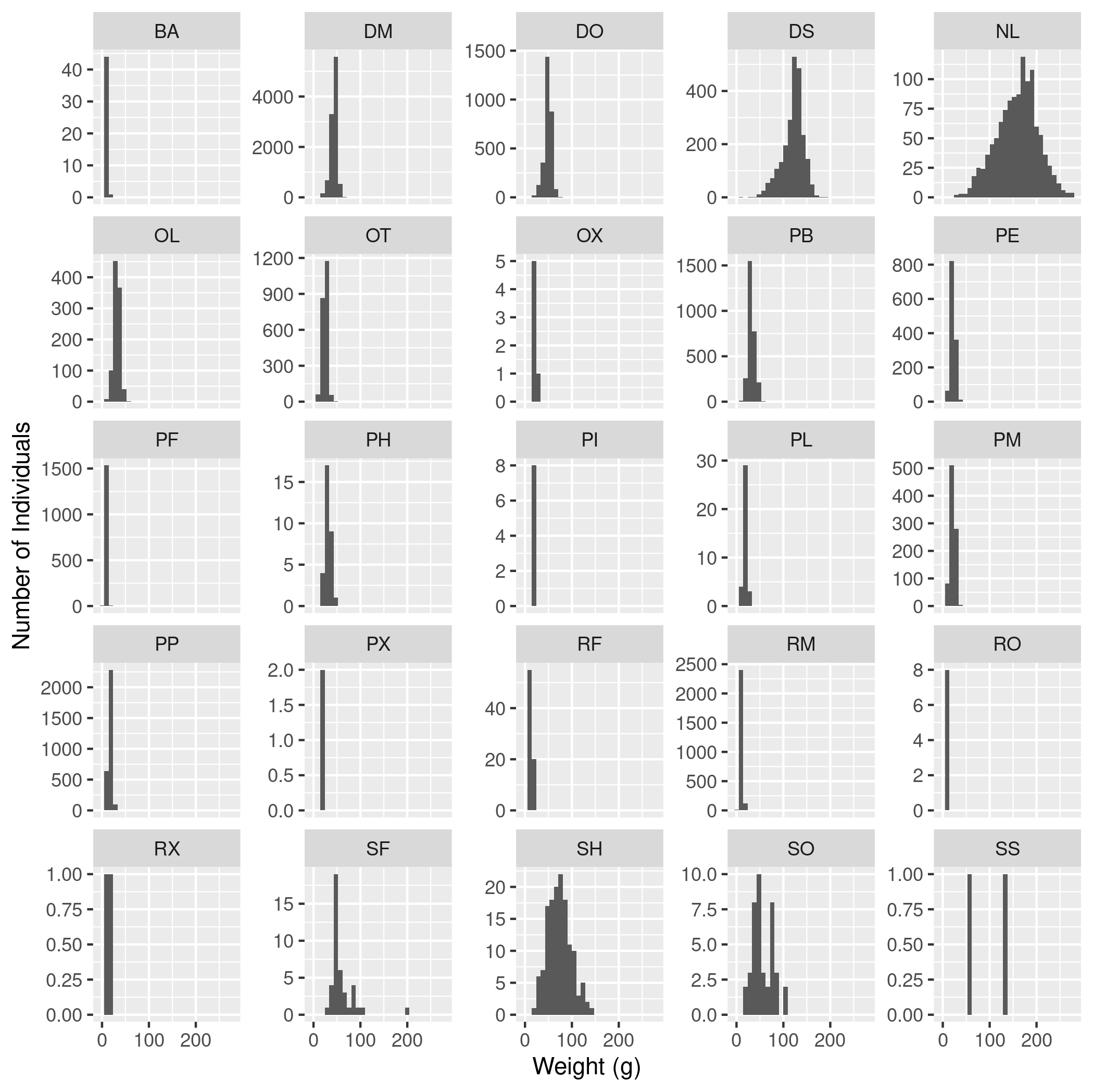
weighton the x-axis andhindfoot_lengthon the y-axis. Use alog10scale on the x-axis. Color the points byspecies_id. Include good axis labels. - Make a histogram of weights with a separate subplot for each
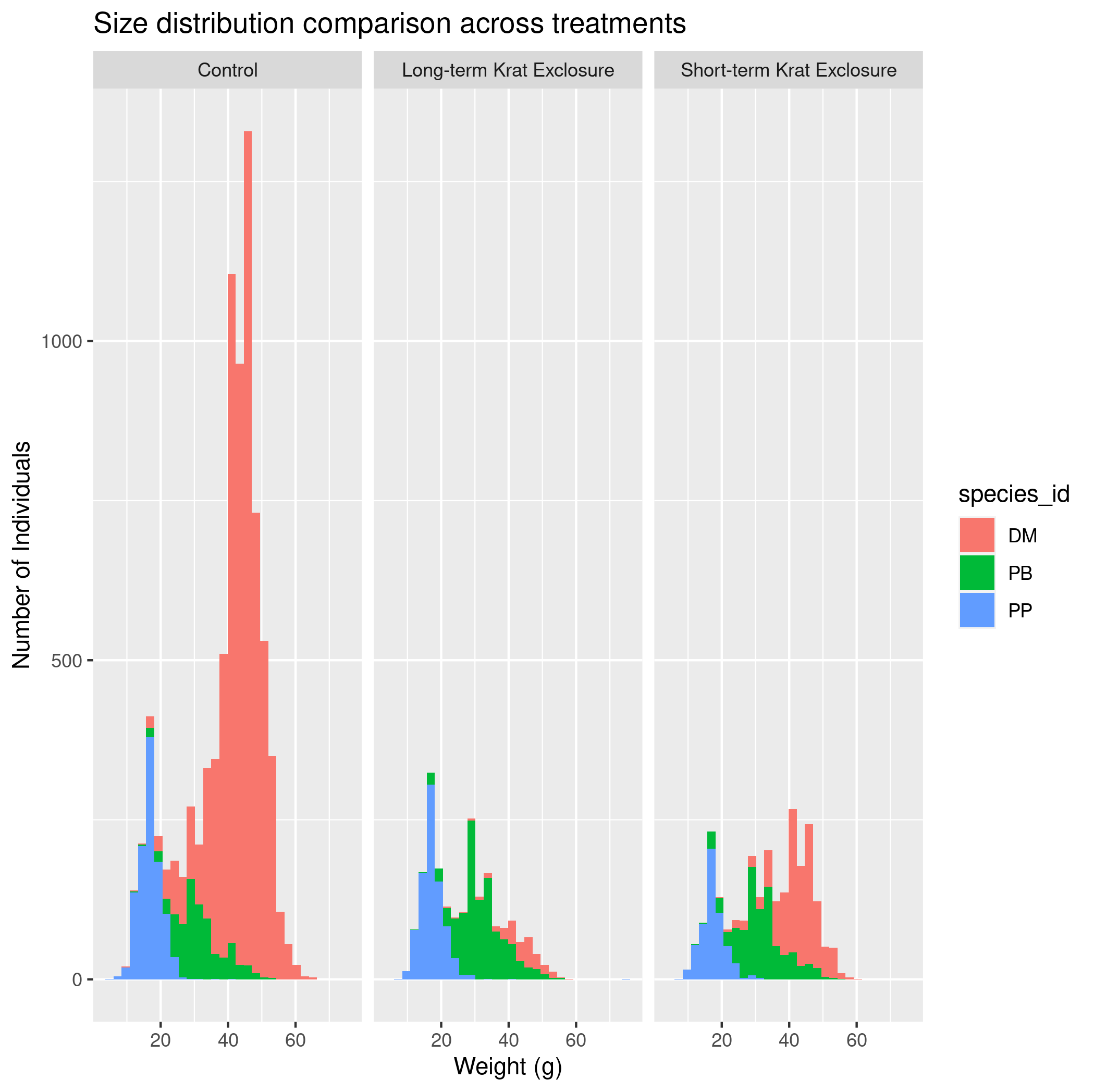
species_id. Do not include species with no weights. Set thescalesargument to"free_y"so that the y-axes can vary. Include good axis labels. - (Challenge) Make a plot with histograms of the weights of three species,
PP,PB, andDM, colored byspecies_id, with a different facet (i.e., subplot) for each of threeplot_type’sControl,Long-term Krat Exclosure, andShort-term Krat Exclosure. Include good axis labels and a title for the plot. Export the plot to apngfile.
- Create a data frame with only data for the
Mammal Body Size (50 pts)
There were a relatively large number of extinctions of mammalian species roughly 10,000 years ago. To help understand why these extinctions happened scientists are interested in understanding whether there were differences in the body size of those species that went extinct and those that did not.
To address this question we can use the “Mammal masses” data on the datasets, which has data on the mass of recently extinct mammals as well as extant mammals (i.e., those that are still alive today). Download the “MOMv3.3.txt” file and put it in your
data/folder.The original dataset is archived on ESA pubs. You can take a look at the metadata to understand the structure of the data. One key thing to remember is that species can occur on more than one continent, and if they do then they will occur more than once in this dataset. Also let’s ignore species that went extinct in the very recent past (designated by the word
"historical"in thestatuscolumn).Import the data into R. If you’ve looked at the raw data file you’ll realize that this dataset is tab delimited. Use the argument
sep = "\t"inread.csv()to properly format the data. There is no header row, so usehead = FALSE.mammal_sizes <- read.csv("data/MOMv3.3.txt", head = FALSE, sep = "\t")Add column names to help identify columns.
colnames(mammal_sizes) <- c("continent", "status", "order",
"family", "genus", "species", "log_mass", "combined_mass",
"reference")
To start let’s explore the data a little and then start looking at the major question.
- The following
dplyrcode will determine how many genera (plural of genus) are in the dataset:nrow(distinct(select(mammal_sizes, genus)))Modify this code into a data wrangling work flow using
dplyrand pipes (%>%or|>) to determine the number of species. Remember that a species is uniquely defined by the combination of its genus name and its species name. Print the result to the screen. The number should be between 4000 and 5000. - Find out how many of the species are extinct and how many are extant, print the result to the screen. HINT: first separate the data into the extinct and extant components and then count the number of species.
- Print out how many families are present in the dataset.
- Now print the genus name, the species name, and the mass of the largest and smallest species (note, it is not possible for a mammal to have negative mass.)
- Calculate the average (i.e., mean) mass of an extinct species and the
average mass of an extant species. The function
mean()should help you here. Don’t worry about species that occur more than once. We’ll consider the values on different continents to represent independent data points.
Print out the results for extinct then extant.
- The following