Learning Objectives
Following this assignment students should be able to:
- use and create vectorized functions
- use the apply family of functions for iteration
- integrate custom functions with dplyr for iteration
Reading
-
Topics
- Iteration
- Style
-
Readings
Lecture Notes
Place this code at the start of the assignment to load all the required packages.
library(dplyr)
library(ggplot2)
Exercises
Size Estimates Vectorized (25 pts)
This is a followup to Use and Modify.
-
Write a function named
mass_from_length_theropoda()that takeslengthas an argument to get an estimate of mass values for the dinosaur Theropoda. Use the equationmass <- 0.73 * length^3.63. Copy the data below into R and pass the entire vector to your function to calculate the estimated mass for each dinosaur.theropoda_lengths <- c(17.8013631070471, 20.3764452071665, 14.0743486294308, 25.65782386974, 26.0952008049675, 20.3111541103134, 17.5663244372533, 11.2563431277577, 20.081903202614, 18.6071626441984, 18.0991894513166, 23.0659685685892, 20.5798853467837, 25.6179254233558, 24.3714331573996, 26.2847248252537, 25.4753783544473, 20.4642089867304, 16.0738256364701, 20.3494171706583, 19.854399305869, 17.7889814608919, 14.8016421998303, 19.6840911485379, 19.4685885050906, 24.4807784966691, 13.3359960054899, 21.5065994598917, 18.4640304608411, 19.5861532398676, 27.084751999756, 18.9609366301798, 22.4829168046521, 11.7325716149514, 18.3758846100456, 15.537504851634, 13.4848751773738, 7.68561192214935, 25.5963348603783, 16.588285389794) -
Create a new version of the function named
mass_from_length()to use the equationmass <- a * length^band takelength,aandbas arguments. In the function arguments, set the default values forato0.73andbto3.63. If you run this function with just the length data from Part 1, you should get the same result as Part 1. Copy the data below into R and call your function using the vector of lengths from Part 1 (above) and these vectors ofaandbvalues to estimate the mass for the dinosaurs using different values ofaandb.a_values <- c(0.759, 0.751, 0.74, 0.746, 0.759, 0.751, 0.749, 0.751, 0.738, 0.768, 0.736, 0.749, 0.746, 0.744, 0.749, 0.751, 0.744, 0.754, 0.774, 0.751, 0.763, 0.749, 0.741, 0.754, 0.746, 0.755, 0.764, 0.758, 0.76, 0.748, 0.745, 0.756, 0.739, 0.733, 0.757, 0.747, 0.741, 0.752, 0.752, 0.748)b_values <- c(3.627, 3.633, 3.626, 3.633, 3.627, 3.629, 3.632, 3.628, 3.633, 3.627, 3.621, 3.63, 3.631, 3.632, 3.628, 3.626, 3.639, 3.626, 3.635, 3.629, 3.642, 3.632, 3.633, 3.629, 3.62, 3.619, 3.638, 3.627, 3.621, 3.628, 3.628, 3.635, 3.624, 3.621, 3.621, 3.632, 3.627, 3.624, 3.634, 3.621) -
Create a data frame for this data using
dino_data <- data.frame(theropoda_lengths, a_values, b_values). Usedplyrto add a newmassescolumn to this data frame (usingmutate()and your function) and print the result to the console.
-
Size Estimates With Maximum (25 pts)
This is a followup to Part 1 Size Estimates Vectorized.
Create a new version of your
Expected outputs for Size Estimates With Maximum: 1mass_from_length_theropoda()function from Part 1 of Size Estimates Vectorized calledmass_from_length_max(). This function should only calculate a mass if the value oflengthpassed to the function is less than 20. Iflengthis greater than 20 returnNAinstead. Usesapply()and this new function to estimate the mass for thetheropoda_lengthsdata from Size Estimates Vectorized.Size Estimates By Name Apply (25 pts)
This is a followup to Size Estimates by Name.
Download the data on dinosaur lengths with species names into your data folder and import it using
read.csv().Write a function
get_mass_from_length_by_name()that uses the equationmass <- a * length^bto estimate the size of a dinosaur from its length. This function should take two arguments, thelengthand the name of the dinosaur group. Inside this function useif/else if/elsestatements to check to see if the name is one of the following values and if so setaandbto the appropriate values.- Stegosauria:
a = 10.95andb = 2.64(Seebacher 2001). - Theropoda:
a = 0.73andb = 3.63(Seebacher 2001). - Sauropoda:
a = 214.44andb = 1.46(Seebacher 2001).
If the name is not any of these values set
a = NAandb = NA.-
Use this function and
mapply()to calculate the estimated mass for each dinosaur. You’ll need to pass the data tomapply()as single vectors or columns, not the whole data frame. -
Using
dplyr, add a newmassescolumn to the data frame (usingrowwise(),mutate()and your function) and print the result to the console. -
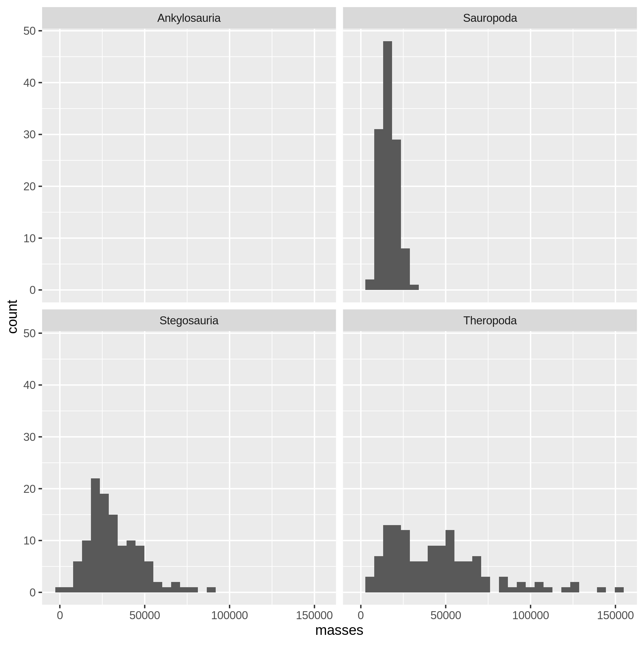
Using
ggplot, make a histogram of dinosaur masses with one subplot for each species (usingfacet_wrap()).
- Stegosauria:
Crown Volume Calculation (25 pts)
The UHURU experiment in Kenya has conducted a survey of Acacia and other tree species in ungulate exclosure treatments. Data for the tree data is available here in a tab delimited (
"\t") format. Each of the individuals surveyed were measured for tree height (HEIGHT) and canopy size in two directions (AXIS_1andAXIS_2). Read these data in using the following code:tree_data <- read.csv("https://ndownloader.figshare.com/files/5629536", sep = '\t', na.strings = c("dead", "missing", "MISSING", "NA", "?", "3.3."))You want to estimate the crown volumes for the different species and have developed equations for species in the Acacia genus:
volume = 0.16 * HEIGHT^0.8 * pi * AXIS_1 * AXIS_2and the Balanites genus:
volume = 1.2 * HEIGHT^0.26 * pi * AXIS_1 * AXIS_2For all other genera you’ll use a general equation developed for trees:
volume = 0.5 * HEIGHT^0.6 * pi * AXIS_1 * AXIS_2-
Write a function called
tree_volume_calcthat calculates the canopy volume for the Acacia species in the dataset. To do so, use an if statement in combination with thestr_detect()function from thestringrR package. The codestr_detect(SPECIES, "Acacia")will returnTRUEif the string stored in this variable contains the word “Acacia” andFALSEif it does not. This function will have to take the following arguments as input: SPECIES, HEIGHT, AXIS_1, AXIS_2. Then run the following line:tree_volume_calc("Acacia_brevispica", 2.2, 3.5, 1.12) -
Expand this function to additionally calculate canopy volumes for other types of trees in this dataset by adding if/else statements and including the volume equations for the Balanites genus and other genera. Then run the following lines:
tree_volume_calc("Balanites", 2.2, 3.5, 1.12)tree_volume_calc("Croton", 2.2, 3.5, 1.12) -
Now get the canopy volumes for all the trees in the
tree_datadataframe and add them as a new column to the data frame. You can do this usingtree_volume_calc()and eithermapply()or usingdplyrwithrowwiseandmutate.
-
Tree Growth (optional)
The UHURU experiment in Kenya has conducted a survey of Acacia and other tree species in ungulate exclosure treatments. Each of the individuals surveyed were measured for tree height (
HEIGHT), circumference (CIRC) and canopy size in two directions (AXIS_1andAXIS_2). If the fileTREE_SURVEYS.txtisn’t already in your working directory, download the data from the data sets menu on the homepage (UHURU tree survey).Read the data in using the following code:
tree_data <- read.csv(here::here("data/TREE_SURVEYS.txt"), sep = '\t', na.strings = c("dead", "missing", "MISSING", "NA", "?", "3.3."), stringsAsFactors = FALSE)-
Write a function named
get_growth()that takes two inputs, a vector ofsizesand a vector ofyears, and calculates the average annual growth rate. Pseudo-code for calculating this rate is(size_in_last_year - size_in_first_year) / (last_year - first_year). Test this function by runningget_growth(c(40.2, 42.6, 46.0), c(2020, 2021, 2022)). -
Use dplyr and this function to get the growth for each individual tree along with information about the
TREATMENTthat tree occurs on. Trees are identified by a unique value in theORIGINAL_TAGcolumn. Don’t include information for cases where aTREATMENTis not known (e.g., where it isNA). -
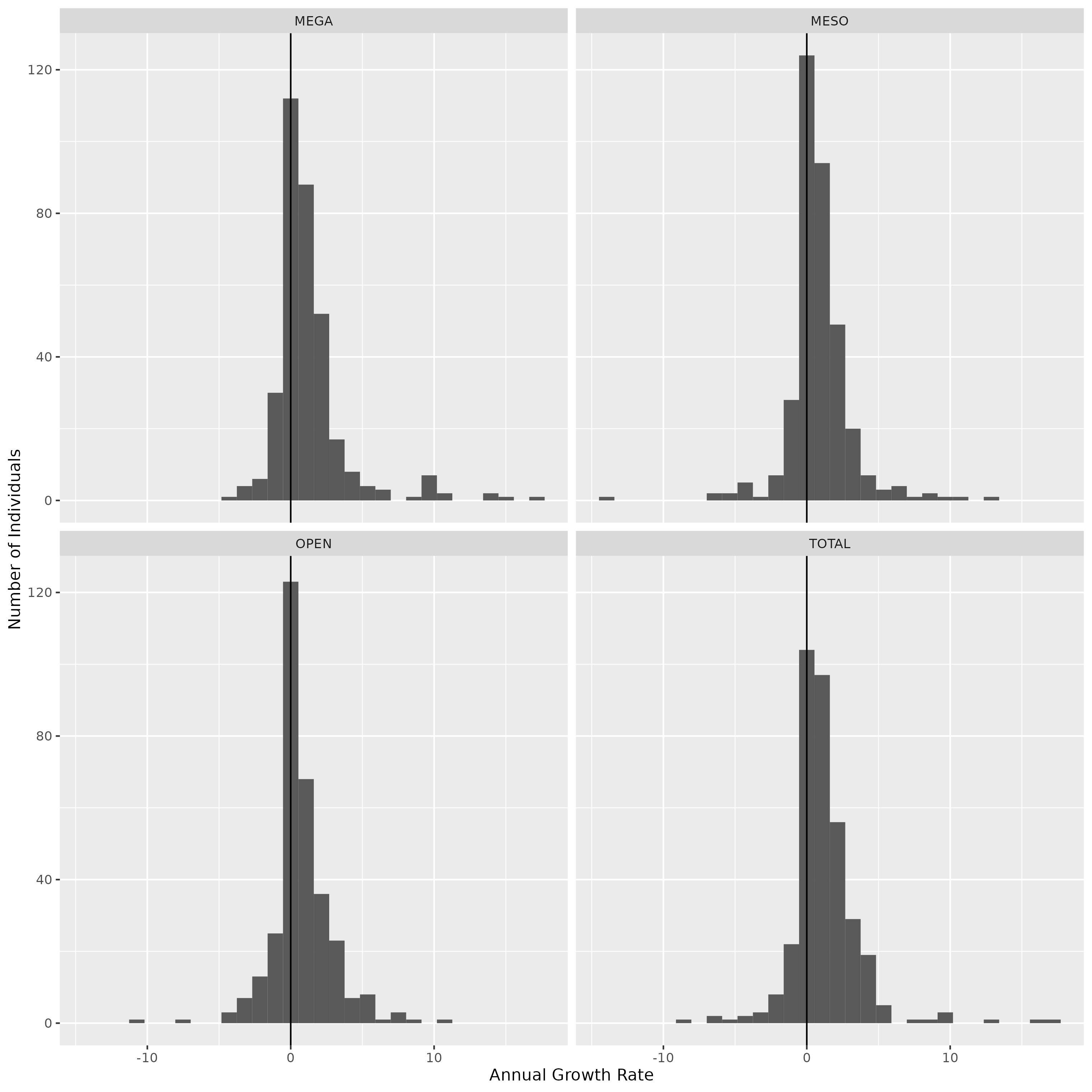
Using ggplot the output from (2) make a histogram of growth rates for each
TREATMENT, which eachTREATMENTin it’s own facet. Usegeom_vline()to add a vertical line at 0 to help indicate which trees are getting bigger vs. smaller. Include good axis labels. -
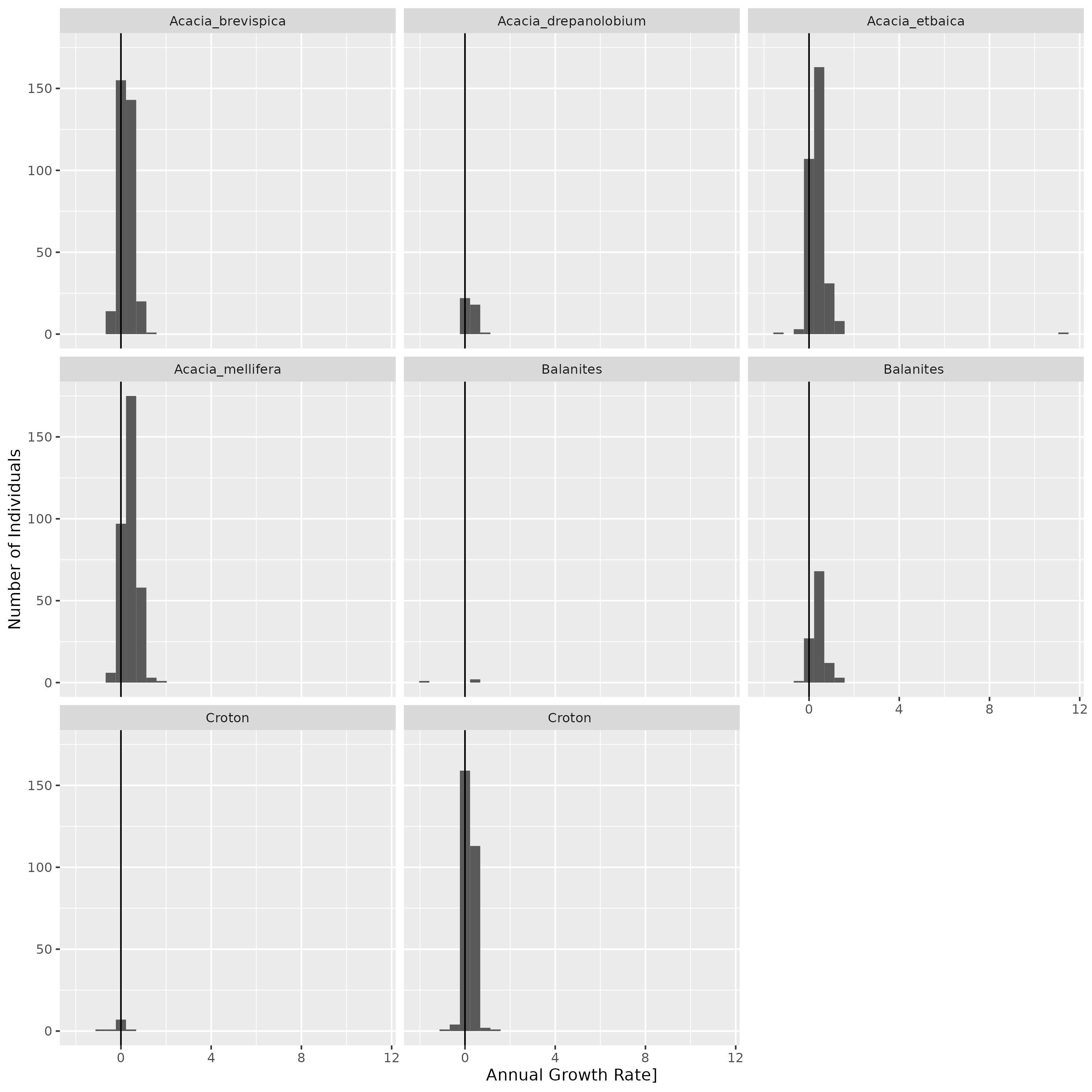
Create a single function called
compare_growth()that combines your work in (2) and (3). It should take the arguments:df(the data frame being used),measure(the column that contains the size measurement to measure growth on; we usedCIRC),tag_column(the name of the column with the unique tag; we usedORIGINAL_TAG),sample_column(the name of the column indicating different samples, we usedYEAR), andfacet_column(the name of the column to use to determine which groups to make histograms for, we usedTREATMENT). Use the function to recreate your original plot usingcompare_growth(tree_data, CIRC, ORIGINAL_TAG, YEAR, TREATMENT). Then use the function to create a similar plot showing growth facetedSPECIES, usingSURVEYas thesample_column, andAXIS_1as themeasureby runningcompare_growth(tree_data, AXIS_1, ORIGINAL_TAG, SURVEY, SPECIES).
-